Running GBTClassifier and GBTRegressor on Hadoop Cluster using Apache Spark's Java API
Gradient-Boosted Trees (GBT) in Apache Spark's MLlib are powerful ensemble learning methods used for both classification and regression tasks. They build a model in a stage-wise fashion, combining multiple weak prediction models (typically decision trees) to create a strong learner.
Both algorithms work by iteratively training a sequence of trees. Each new tree is trained to correct the errors made by the previous ones. The key difference lies in the loss function they are designed to minimize.
This article will explore the implementation of supervised machine learning tasks utilizing the Java language alongside Apache Spark's scalable machine learning library (MLlib). We will demonstrate how to construct robust, distributed learning models that run efficiently on a Hadoop cluster
The process will leverage the core strengths of each technology in a modern big data architecture:
- Java provides a powerful, type-safe, and high-performance foundation for developing enterprise-grade Spark applications.
- Apache Spark MLlib offers a distributed framework for machine learning, enabling the training of models on massive datasets that far exceed the memory of a single machine.
- The Hadoop Cluster (specifically HDFS - Hadoop Distributed File System) acts as the reliable and scalable storage layer, ensuring our large datasets are available across all nodes for parallel processing.
We will guide you through the complete workflow—from data ingestion stored in HDFS to model training and evaluation—showcasing how to harness the combined power of Java and Spark to solve predictive analytics problems at scale.
This project outlines the development of predictive both Classification and regression models using a modern big data stack We will leverage the scalability of Hadoop 3.3.0 for distributed storage and the high-performance processing engine of Spark 3.1.1 for in-memory analytics. Our goal is to build and evaluate Gradient-Boosted Trees (GBT) model using a classic dataset: the yellow_tripdata_2014-08.csv file, which contains records of New York City yellow taxi trips for August 2014.

Image by Bishnu Sarangi from Pixabay
If you are interested with the data you can collect it from here Click the link. Yellow NYC taxi trip Data . For Classification method, our task is to implement a model to predict for a given taxi trip, if a tip will be paid or not for a trip. And for Regression method, our task is to implement a model to predict for a given taxi trip, what is the expected tip amount for a trip. Our Hadoop environment is three nodes cluster, one namenode and two datanodes.
Here we will use Java 8 and IntelliJ IDEA for this module. Our essential Maven dependency commands of pom.xml are as following
        <dependency>
            <groupId>org.apache.spark</groupId>
            <artifactId>spark-core_2.12</artifactId>
            <version>3.1.1</version>
        </dependency>
        <dependency>
            <groupId>org.apache.spark</groupId>
            <artifactId>spark-sql_2.12</artifactId>
            <version>3.1.1</version>
            <scope>provided</scope>
        </dependency>
        <dependency>
            <groupId>org.apache.spark</groupId>
            <artifactId>spark-mllib_2.12</artifactId>
            <version>3.1.1</version>
            <scope>provided</scope>
        </dependency>
        <dependency>
            <groupId>org.jfree</groupId>
            <artifactId>jfreechart</artifactId>
            <version>1.5.3</version>
        </dependency>
Import libraries
The Spark, ML, and other libraries we'll need by using the following lines of code
        import org.apache.spark.api.java.JavaRDD;
        import org.apache.spark.api.java.function.Function;
        import org.apache.spark.ml.Pipeline;
        import org.apache.spark.ml.PipelineModel;
        import org.apache.spark.ml.PipelineStage;
        import org.apache.spark.ml.classification.GBTClassifier;
        import org.apache.spark.ml.evaluation.BinaryClassificationEvaluator;
        import org.apache.spark.ml.evaluation.MulticlassClassificationEvaluator;
        import org.apache.spark.ml.evaluation.RegressionEvaluator;
        import org.apache.spark.ml.feature.*;
        import org.apache.spark.ml.regression.GBTRegressor;
        import org.apache.spark.mllib.evaluation.RegressionMetrics;
        import org.apache.spark.sql.*;
        import org.apache.spark.sql.types.DataTypes;
        import org.apache.spark.sql.types.StructField;
        import org.apache.spark.sql.types.StructType;
        import org.jfree.chart.*;
        import org.jfree.chart.plot.CategoryPlot;
        import org.jfree.chart.plot.PlotOrientation;
        import org.jfree.chart.plot.XYPlot;
        import org.jfree.chart.renderer.xy.XYShapeRenderer;
        import org.jfree.data.category.DefaultCategoryDataset;
        import org.jfree.data.statistics.DefaultBoxAndWhiskerCategoryDataset;
        import org.jfree.data.statistics.HistogramDataset;
        import org.jfree.data.statistics.HistogramType;
        import org.jfree.data.xy.XYSeries;
        import org.jfree.data.xy.XYSeriesCollection;
        import scala.Tuple2;

        import javax.swing.*;
        import java.awt.*;
        import java.io.File;
        import java.io.IOException;
        import java.util.ArrayList;
        import java.util.List;
Data Exploration
At first we ingest the data that we want to analyze. The data is brought from external sources or systems where it resides into data exploration and modeling environment. The data exploration and modeling environment is Spark. Firstly we need to make sure our source of data that is our dataset files are present in HDFS where we expect to read them from our spark jobs. To put the files in HDFS first bring the files to the operating system i.e. Linux in our case and from Linux we copy them to HDFS using the following command
We will first load dataset using Apache Spark and see the total numbers of rows, header, and first 5 rows of our dataset. For these our lines of codes are shown bellow
            SparkSession spark = SparkSession
                    .builder()
                    .master("local[*]")
                    .appName("NycTripApp")
                    .getOrCreate();

            JavaRDD<String> dataRaw = spark.sparkContext()
                    .textFile("hdfs://master:9000/data/data/yellow_tripdata_2014-08.csv",1).toJavaRDD();
            String header = dataRaw.first();
Now we print the header of the dataset.
System.out.println(header);
Output:
vendor_id, pickup_datetime, dropoff_datetime, passenger_count, trip_distance, pickup_longitude, pickup_latitude, rate_code, store_and_fwd_flag, dropoff_longitude, dropoff_latitude, payment_type, fare_amount, surcharge, mta_tax, tip_amount, tolls_amount, total_amount
Total numbers of records of Dataset
System.out.println("Total Records : " + dataRaw.count());
Output:
Total Records : 12688879
The code of first 5 rows of the dataset is as follows
dataRaw.take(5).forEach(s -> System.out.println(s));
OutPut:
        vendor_id, pickup_datetime, dropoff_datetime, passenger_count, trip_distance, pickup_longitude, pickup_latitude, rate_code, store_and_fwd_flag, dropoff_longitude, dropoff_latitude, payment_type, fare_amount, surcharge, mta_tax, tip_amount, tolls_amount, total_amount

        CMT,2014-08-16 14:58:49,2014-08-16 15:15:59,1,2.7000000000000002,-73.946537000000006,40.776812999999997,1,N,-73.976192999999995,40.755625000000002,CSH,14,0,0.5,0,0,14.5
        CMT,2014-08-16 08:10:48,2014-08-16 08:58:16,3,20.399999999999999,-73.776857000000007,40.645099000000002,1,Y,-73.916248999999993,40.837356999999997,CSH,58.5,0,0.5,0,5.3300000000000001,64.329999999999998
        CMT,2014-08-16 09:44:07,2014-08-16 09:54:37,1,2.1000000000000001,-73.986585000000005,40.725847999999999,1,N,-73.977157000000005,40.751961000000001,CSH,9.5,0,0.5,0,0,10
Now we can see the dataset rows printed above, We loaded the dataset from an HDFS location and stored it in an RDD of strings. Fortunately, the dataset is relatively clean and has one row per data item but it contains a empty row. Next, we remove the header, delete the empty row and again print 5 rows from the dataset, we run the codes following
            JavaRDD<String> dataLines = dataRaw.filter( row -> {
                    return !row.contains("vendor_id") && !row.isEmpty();
                   });
            dataLines.take(5).forEach(s -> System.out.println(s));
Output:
        CMT,2014-08-16 14:58:49,2014-08-16 15:15:59,1,2.7000000000000002,-73.946537000000006,40.776812999999997,1,N,-73.976192999999995,40.755625000000002,CSH,14,0,0.5,0,0,14.5
        CMT,2014-08-16 08:10:48,2014-08-16 08:58:16,3,20.399999999999999,-73.776857000000007,40.645099000000002,1,Y,-73.916248999999993,40.837356999999997,CSH,58.5,0,0.5,0,5.3300000000000001,64.329999999999998
        CMT,2014-08-16 09:44:07,2014-08-16 09:54:37,1,2.1000000000000001,-73.986585000000005,40.725847999999999,1,N,-73.977157000000005,40.751961000000001,CSH,9.5,0,0.5,0,0,10
        CMT,2014-08-16 10:46:13,2014-08-16 10:51:25,1,1.3,-73.976290000000006,40.765231,1,N,-73.961484999999996,40.777889000000002,CSH,6,0,0.5,0,0,6.5
        CMT,2014-08-16 09:27:23,2014-08-16 09:39:37,2,1.7,-73.995248000000004,40.754646000000001,1,Y,-73.995902999999998,40.769201000000002,CSH,10.5,0,0.5,0,0,11
As seen, the rows of dataset are fine, now we generate schema based on the column strings of the header of the dataset, cast variables according to the schema, and create an initial dataframe and lastly see 10 rows of the dataset, for these we run the following lines of codes
        List<StructField> fields = new ArrayList<>();
        fields.add(DataTypes.createStructField("vendor_id", DataTypes.StringType, true));
        fields.add(DataTypes.createStructField("pickup_datetime", DataTypes.StringType, true));
        fields.add(DataTypes.createStructField("dropoff_datetime", DataTypes.StringType, true));
        fields.add(DataTypes.createStructField("passenger_count", DataTypes.DoubleType, true));
        fields.add(DataTypes.createStructField("trip_distance", DataTypes.DoubleType, true));
        fields.add(DataTypes.createStructField("pickup_longitude", DataTypes.DoubleType, true));
        fields.add(DataTypes.createStructField("pickup_latitude", DataTypes.DoubleType, true));
        fields.add(DataTypes.createStructField("rate_code", DataTypes.DoubleType, true));
        fields.add(DataTypes.createStructField("store_and_fwd_flag", DataTypes.StringType, true));
        fields.add(DataTypes.createStructField("dropoff_longitude", DataTypes.DoubleType, true));
        fields.add(DataTypes.createStructField("dropoff_latitude", DataTypes.DoubleType, true));
        fields.add(DataTypes.createStructField("payment_type", DataTypes.StringType, true));
        fields.add(DataTypes.createStructField("fare_amount", DataTypes.DoubleType, true));
        fields.add(DataTypes.createStructField("surcharge", DataTypes.DoubleType, true));
        fields.add(DataTypes.createStructField("mta_tax", DataTypes.DoubleType, true));
        fields.add(DataTypes.createStructField("tip_amount", DataTypes.DoubleType, true));
        fields.add(DataTypes.createStructField("tolls_amount", DataTypes.DoubleType, true));
        fields.add(DataTypes.createStructField("total_amount", DataTypes.DoubleType, true));

        StructType schema = DataTypes.createStructType(fields);
        JavaRDD<Row> rowRDD = dataLines.map((Function<String, Row>) row -> {
        String[] arr = row.split(",");
        return RowFactory.create(
        arr[0], arr[1], arr[2],
        Double.parseDouble(arr[3].trim()), Double.parseDouble(arr[4].trim()),
        Double.parseDouble(arr[5].trim()), Double.parseDouble(arr[6].trim()),
        Double.parseDouble(arr[7].trim()), arr[8],
        Double.parseDouble(arr[9].trim()), Double.parseDouble(arr[10].trim()),
        arr[11], Double.parseDouble(arr[12].trim()),
        Double.parseDouble(arr[13].trim()), Double.parseDouble(arr[14].trim()),
        Double.parseDouble(arr[15].trim()), Double.parseDouble(arr[16].trim()),
        Double.parseDouble(arr[17].trim()));
        });

        Dataset<Row> dataDF = spark.createDataFrame(rowRDD, schema);
        dataDF.show(10);
Output:
        +---------+-------------------+-------------------+---------------+-------------+----------------+---------------+---------+------------------+-----------------+----------------+------------+-----------+---------+-------+----------+------------+------------+
        |vendor_id|    pickup_datetime|   dropoff_datetime|passenger_count|trip_distance|pickup_longitude|pickup_latitude|rate_code|store_and_fwd_flag|dropoff_longitude|dropoff_latitude|payment_type|fare_amount|surcharge|mta_tax|tip_amount|tolls_amount|total_amount|
        +---------+-------------------+-------------------+---------------+-------------+----------------+---------------+---------+------------------+-----------------+----------------+------------+-----------+---------+-------+----------+------------+------------+
        |      CMT|2014-08-16 14:58:49|2014-08-16 15:15:59|            1.0|          2.7|      -73.946537|      40.776813|      1.0|                 N|       -73.976193|       40.755625|         CSH|       14.0|      0.0|    0.5|       0.0|         0.0|        14.5|
        |      CMT|2014-08-16 08:10:48|2014-08-16 08:58:16|            3.0|         20.4|      -73.776857|      40.645099|      1.0|                 Y|       -73.916249|       40.837357|         CSH|       58.5|      0.0|    0.5|       0.0|        5.33|       64.33|
        |      CMT|2014-08-16 09:44:07|2014-08-16 09:54:37|            1.0|          2.1|      -73.986585|      40.725848|      1.0|                 N|       -73.977157|       40.751961|         CSH|        9.5|      0.0|    0.5|       0.0|         0.0|        10.0|
        |      CMT|2014-08-16 10:46:13|2014-08-16 10:51:25|            1.0|          1.3|       -73.97629|      40.765231|      1.0|                 N|       -73.961485|       40.777889|         CSH|        6.0|      0.0|    0.5|       0.0|         0.0|         6.5|
        |      CMT|2014-08-16 09:27:23|2014-08-16 09:39:37|            2.0|          1.7|      -73.995248|      40.754646|      1.0|                 Y|       -73.995903|       40.769201|         CSH|       10.5|      0.0|    0.5|       0.0|         0.0|        11.0|
        |      CMT|2014-08-16 14:14:16|2014-08-16 14:25:33|            2.0|          1.7|      -73.991535|      40.759863|      1.0|                 N|       -74.005722|       40.737558|         CSH|       10.0|      0.0|    0.5|       0.0|         0.0|        10.5|
        |      CMT|2014-08-16 15:55:16|2014-08-16 16:00:10|            1.0|          1.0|      -73.972307|      40.794076|      1.0|                 N|       -73.963865|       40.807858|         CSH|        6.0|      0.0|    0.5|       0.0|         0.0|         6.5|
        |      CMT|2014-08-16 14:08:29|2014-08-16 14:32:03|            1.0|          9.2|      -73.967338|      40.766009|      1.0|                 N|       -73.872972|       40.774487|         CSH|       28.5|      0.0|    0.5|       0.0|         0.0|        29.0|
        |      CMT|2014-08-16 11:11:21|2014-08-16 11:23:48|            1.0|          2.6|      -73.973775|      40.794591|      1.0|                 N|       -73.970561|       40.768086|         CSH|       11.5|      0.0|    0.5|       0.0|         0.0|        12.0|
        |      CMT|2014-08-16 07:44:56|2014-08-16 07:49:26|            1.0|          1.4|       -73.98636|      40.737913|      1.0|                 N|       -73.977117|       40.751126|         CSH|        6.0|      0.0|    0.5|       0.0|         0.0|         6.5|
        +---------+-------------------+-------------------+---------------+-------------+----------------+---------------+---------+------------------+-----------------+----------------+------------+-----------+---------+-------+----------+------------+------------+
        only showing top 10 rows
We are not interested with all the columns of the dataset, we create a cleaned data frame by droping unwanted columns and filtering unwanted values, cache and materialize the data frame in memory, and register the cleaned data frame as a temporary table in sqlcontext.
        Dataset<Row> dataDF_cleaned = dataDF
        .drop(dataDF.col("store_and_fwd_flag"))
        .drop(dataDF.col("pickup_datetime")).drop(dataDF.col("dropoff_datetime"))
        .drop(dataDF.col("pickup_longitude")).drop(dataDF.col("pickup_latitude"))
        .drop(dataDF.col("dropoff_longitude")).drop(dataDF.col("dropoff_latitude"))
        .drop(dataDF.col("surcharge")).drop(dataDF.col("mta_tax"))
        .drop(dataDF.col("total_amount")).drop(dataDF.col("tolls_amount"))
        .filter("passenger_count > 0 AND fare_amount >= 1 AND trip_distance > 0 ");

        dataDF_cleaned.cache();
        dataDF_cleaned.createOrReplaceTempView("tempView");
Data Visualization
In this section, we examine the data by using SQL queries and import the results into a data frame to plot the target variables and prospective features for visual inspection by using the automatic visualization. Here we are using JFreeChart 1.5.3 for graphical data representations.
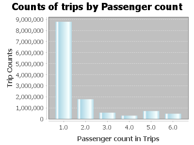
Counts of trips by passenger
        Dataset<Row> plotDF1 = spark.sql("Select passenger_count, COUNT(*) AS trip_counts " +
        "FROM tempView " +
        "WHERE passenger_count > 0 and passenger_count < 7 " +
        "GROUP BY passenger_count Order by passenger_count");

        List<Row> rows = plotDF1.collectAsList();

        DefaultCategoryDataset dataset = new DefaultCategoryDataset();

        for (Row row : rows) {
            double passengerCount = row.getDouble(0);
            long tripCounts = row.getLong(1);
            dataset.addValue(tripCounts, "Trip Counts", String.valueOf(passengerCount));
        }

        JFreeChart chart = ChartFactory.createBarChart(
                "Counts of trips by Passenger count",
                "Passenger count in Trips",
                "Trip Counts",
                dataset,
                PlotOrientation.VERTICAL,
                false,
                true,
                false
        );

        chart.getCategoryPlot().getRenderer().setSeriesPaint(0, new java.awt.Color(173, 216, 230)); // lightblue

        ChartFrame frame = new ChartFrame("Passenger Count Visualization", chart);
        frame.pack();
        frame.setVisible(true);
Output:

SQL Query and Data frame:
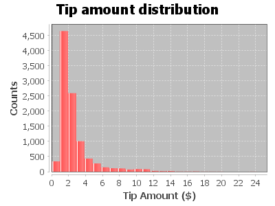
        Dataset<Row> plotDF2 = spark.sql(
                "SELECT fare_amount, passenger_count, tip_amount " +
                        "FROM tempView " +
                        "WHERE passenger_count > 0 AND passenger_count < 7 AND " +
                        "fare_amount > 0 AND fare_amount < 200 AND payment_type in ('CSH', 'CRD') AND " +
                        "tip_amount > 0 AND tip_amount < 25 " +
                        "limit 10000"
        );
        List<Row> tipAmounts = plotDF2.select("tip_amount").collectAsList();
        double[] tipValues = new double[tipAmounts.size()];
        for (int i = 0; i < tipAmounts.size(); i++) {
            tipValues[i] = tipAmounts.get(i).getDouble(0);
        }
        HistogramDataset dataset = new HistogramDataset();
        dataset.setType(HistogramType.FREQUENCY);
        dataset.addSeries("Tip Amount", tipValues, 25); // 25 bins as in the Python code
        JFreeChart histogram = ChartFactory.createHistogram(
                "Tip amount distribution",
                "Tip Amount ($)",
                "Counts",
                dataset,
                PlotOrientation.VERTICAL,
                false,
                true,
                false
        );
        ChartFrame frame = new ChartFrame("Tip Amount Distribution", histogram);
        frame.pack();
        frame.setVisible(true);
Histogram of tip amount
Output:
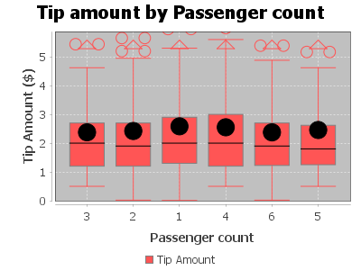
Relationship between tip amount and Passenger Count
        Dataset<Row> plotDF2 = spark.sql(
                "SELECT fare_amount, passenger_count, tip_amount " +
                        "FROM tempView " +
                        "WHERE passenger_count > 0 AND passenger_count < 7 AND " +
                        "fare_amount > 0 AND fare_amount < 200 AND payment_type in ('CSH', 'CRD') AND " +
                        "tip_amount > 0 AND tip_amount < 25 " +
                        "limit 10000"
        );
        List<Row> grouped = plotDF2.groupBy("passenger_count")
                .agg(functions.collect_list("tip_amount").alias("tips"))
                .collectAsList();

        DefaultBoxAndWhiskerCategoryDataset dataset = new DefaultBoxAndWhiskerCategoryDataset();

        for (Row row : grouped) {
            double passengerCount = row.getDouble(0);
            List<Double> tips = row.getList(1);
            dataset.add(tips, "Tip Amount", String.valueOf((int) passengerCount));
        }
        JFreeChart chart = ChartFactory.createBoxAndWhiskerChart(
                "Tip amount by Passenger count",
                "Passenger count",
                "Tip Amount ($)",
                dataset,
                true
        );
        CategoryPlot plot = (CategoryPlot) chart.getPlot();
        plot.setDomainGridlinesVisible(true);
        plot.setRangeGridlinesVisible(true);

        JFrame frame = new JFrame("Boxplot");
        frame.setContentPane(new ChartPanel(chart));
        frame.setSize(800, 600);
        frame.setVisible(true);
        frame.setDefaultCloseOperation(JFrame.EXIT_ON_CLOSE);
Output:
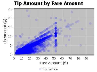
Relationship between tip amount and Fare Amount
        Dataset<Row> plotDF = spark.sql(
                "SELECT fare_amount, passenger_count, tip_amount " +
                        "FROM tempView " +
                        "WHERE passenger_count > 0 AND passenger_count < 7 AND " +
                        "fare_amount > 0 AND fare_amount < 200 AND " +
                        "payment_type IN ('CSH', 'CRD') AND " +
                        "tip_amount > 0 AND tip_amount < 25 " +
                        "LIMIT 10000"
        );
        List<Row> rows = plotDF.collectAsList();
        XYSeries series = new XYSeries("Tips vs Fare");
        for (Row r : rows) {
            double fare = r.getAs("fare_amount");
            double tip = r.getAs("tip_amount");
            series.add(fare, tip);
        }
        XYSeriesCollection dataset = new XYSeriesCollection(series);
        JFreeChart scatterPlot = ChartFactory.createScatterPlot(
                "Tip Amount by Fare Amount",
                "Fare Amount ($)",
                "Tip Amount ($)",
                dataset,
                PlotOrientation.VERTICAL,
                true,
                true,
                false
        );
        XYPlot plot = (XYPlot) scatterPlot.getPlot();
        XYShapeRenderer renderer = new XYShapeRenderer();
        renderer.setSeriesPaint(0, new Color(0, 0, 255, 30));
        plot.setRenderer(renderer);
        SwingUtilities.invokeLater(() -> {
            JFrame frame = new JFrame("Scatter Plot Example");
            frame.setDefaultCloseOperation(JFrame.EXIT_ON_CLOSE);
            frame.add(new ChartPanel(scatterPlot));
            frame.setSize(800, 600);
            frame.setLocationRelativeTo(null);
            frame.setVisible(true);
        });
Output:
Feature engineering, transformation and data preparation for modeling
Next, we create a new feature tipped, if the tip_amount is non-zero, then this returns 1, else 0 in our case. We build a classifier with this target value later on.
        String sqlStatement = "SELECT *, " +
                "CASE " +
                "WHEN tip_amount > 0  THEN 1 ELSE 0 END as tipped " +
                "FROM tempView";

        Dataset<Row> data_newFeature = spark.sql(sqlStatement);
        data_newFeature.show();
Output:
        +---------+---------------+-------------+---------+------------+-----------+----------+------+
        |vendor_id|passenger_count|trip_distance|rate_code|payment_type|fare_amount|tip_amount|tipped|
        +---------+---------------+-------------+---------+------------+-----------+----------+------+
        |      CMT|            1.0|          2.7|      1.0|         CSH|       14.0|       0.0|     0|
        |      CMT|            3.0|         20.4|      1.0|         CSH|       58.5|       0.0|     0|
        |      CMT|            1.0|          2.1|      1.0|         CSH|        9.5|       0.0|     0|
        |      CMT|            1.0|          1.3|      1.0|         CSH|        6.0|       0.0|     0|
        |      CMT|            2.0|          1.7|      1.0|         CSH|       10.5|       0.0|     0|
        |      CMT|            2.0|          1.7|      1.0|         CSH|       10.0|       0.0|     0|
        |      CMT|            1.0|          1.0|      1.0|         CSH|        6.0|       0.0|     0|
        |      CMT|            1.0|          9.2|      1.0|         CSH|       28.5|       0.0|     0|
        |      CMT|            1.0|          2.6|      1.0|         CSH|       11.5|       0.0|     0|
        |      CMT|            1.0|          1.4|      1.0|         CSH|        6.0|       0.0|     0|
        |      CMT|            4.0|          3.2|      1.0|         CSH|       13.0|       0.0|     0|
        |      CMT|            1.0|          7.8|      1.0|         CSH|       25.0|       0.0|     0|
        |      CMT|            1.0|          1.1|      1.0|         CSH|        5.5|       0.0|     0|
        |      CMT|            1.0|          3.3|      1.0|         CSH|       15.5|       0.0|     0|
        |      CMT|            1.0|          5.3|      1.0|         CSH|       19.5|       0.0|     0|
        |      CMT|            1.0|          6.2|      1.0|         CSH|       19.5|       0.0|     0|
        |      CMT|            1.0|         15.6|      2.0|         CSH|       52.0|       0.0|     0|
        |      CMT|            2.0|          0.9|      1.0|         CSH|        6.0|       0.0|     0|
        |      CMT|            1.0|          1.4|      1.0|         CSH|        9.0|       0.0|     0|
        |      CMT|            2.0|          1.2|      1.0|         CSH|        7.0|       0.0|     0|
        +---------+---------------+-------------+---------+------------+-----------+----------+------+
        only showing top 20 rows
Now, we figure out the average, minimum, maximum, etc. of columns, as this give us general idea about the range of values and other statistics. Apache Spark SQL provides us with a handy describe method that will help us to calculate these values.
data_newFeature.describe("passenger_count","trip_distance", "rate_code", "fare_amount","tip_amount").show();
Output:
        +-------+------------------+------------------+-------------------+------------------+------------------+
        |summary|   passenger_count|     trip_distance|          rate_code|       fare_amount|        tip_amount|
        +-------+------------------+------------------+-------------------+------------------+------------------+
        |  count|          12612051|          12612051|           12612051|          12612051|          12612051|
        |   mean| 1.711963105762893| 3.081084886986297| 1.0316361708337525|12.782634287634899|1.4699661752082924|
        | stddev|1.3616351834672402|3.6140504506213844|0.28838467968053266|10.461028944648847| 2.272277866399201|
        |    min|               1.0|              0.01|                0.0|               2.5|               0.0|
        |    max|               9.0|             100.0|              221.0|             500.0|             200.0|
        +-------+------------------+------------------+-------------------+------------------+------------------+
Finally, let's use the StringIndexer and create the label for the dataset, we provide the input column and the indexer will read the data and generate output:
        StringIndexerModel labelIndexer = new StringIndexer()
                  .setInputCol("tipped")
                  .setOutputCol("indexedtippedLabel")
                  .fit(data_newFeature);
The dataset contains categorical fields: vendor_id, rate_code, and payment_type. Therefore, we need to convert these into indexed fields, because our models are mathematical and understand only numerical values.To do this, we will use a handy StringIndexerModel provide by Apache Saprk features package.
        StringIndexerModel vendor_idIndexer = new StringIndexer()
                .setInputCol("vendor_id")
                .setOutputCol("vendor_idIndex")
                .fit(data_newFeature);
        Dataset<Row> Indexedvendor_id = vendor_idIndexer.transform(data_newFeature);

        StringIndexerModel rate_codeIndexer = new StringIndexer()
                .setInputCol("rate_code")
                .setOutputCol("rate_codeIndex")
                .fit(Indexedvendor_id);
        Dataset<Row> Indexedrate_code = rate_codeIndexer.transform(Indexedvendor_id);

        StringIndexerModel payment_typeIndexer = new StringIndexer()
                .setInputCol("payment_type")
                .setOutputCol("payment_typeIndex")
                .fit(Indexedrate_code);
        Dataset<Row> IndexedFinal = payment_typeIndexer.transform(Indexedrate_code);
        //IndexedFinal.show();
Now, we use VectorAssembler which is a transformer that combines a given list of columns into a single vector column. It is useful for combining raw features and features generated by different feature transformers into a single feature vector, in order to train ML models, VectorAssembler accepts the input column, in each row, the values of the input columns will be concatenated into a vector in the specified order.
        String[] featuresArr =
                {"vendor_idIndex", "rate_codeIndex", "payment_typeIndex", "passenger_count", "trip_distance", "fare_amount"};

        VectorAssembler va = new VectorAssembler().setInputCols(featuresArr).setOutputCol("features");
Gradient-boosted tree classifier:
This code creates a 25% random sampling of the data in this example. Next, split the sample into a training part (75%, in this example) and a testing part (25%, in this example) to use in classification and regression modeling.
        //Sampling and splitting fractions
        Double samplingFraction = 0.25;
        Double trainingFraction = 0.75;
        Double testingFraction = (1-trainingFraction);
        int seed = 1234;

        Dataset<Row> FinalSampled = data_newFeature.sample(false, samplingFraction, seed = seed);
        //System.out.println("Total : " + FinalSampled.count());

        Dataset<Row> [] splits = FinalSampled.randomSplit(new double[] {trainingFraction, testingFraction});
        Dataset<Row> trainData = splits[0];
        Dataset<Row> testData = splits[1];
        // trainData.show();
Next, we create a GBT classification model by using ML's GBTClassifier() function and convert indexed labels back to original labels.
        GBTClassifier GBT_Classifier = new GBTClassifier()
                .setLabelCol("indexedtippedLabel")
                .setFeaturesCol("features")
                .setMaxIter(10);

        IndexToString labelConverter = new IndexToString()
                .setInputCol("prediction")
                .setOutputCol("predictedtippedLabel")
                .setLabels(labelIndexer.labelsArray()[0]);
Now, A Pipeline chains multiple workflows together to specify an ML workflow, the model is trained with training data and then evaluated on test data. Finally we select examples rows of the evaluated dataset.
        Pipeline pipeline_GBT_Classifier = new Pipeline()
                .setStages(new PipelineStage[] {labelIndexer, va, GBT_Classifier, labelConverter});

        PipelineModel model_GBT_Classifier = pipeline_GBT_Classifier.fit(trainData);
        Dataset<Row> predictions_GBT_Classifier = model_GBT_Classifier.transform(testData);
        //predictions_GBT_Classifier.show();

        predictions_GBT_Classifier.select("predictedtippedLabel","tipped","features").show();
Output:
        +--------------------+------+--------------------+
        |predictedtippedLabel|tipped|            features|
        +--------------------+------+--------------------+
        |                   1|     1|[1.0,0.0,0.0,1.0,...|
        |                   1|     1|[1.0,0.0,0.0,1.0,...|
        |                   1|     1|[1.0,0.0,0.0,1.0,...|
        |                   0|     0|[1.0,0.0,1.0,1.0,...|
        |                   0|     0|[1.0,0.0,1.0,1.0,...|
        |                   0|     0|[1.0,0.0,1.0,1.0,...|
        |                   0|     0|[1.0,0.0,1.0,1.0,...|
        |                   0|     0|[1.0,0.0,1.0,1.0,...|
        |                   0|     0|[1.0,0.0,1.0,1.0,...|
        |                   0|     0|[1.0,0.0,1.0,1.0,...|
        |                   0|     0|[1.0,0.0,1.0,1.0,...|
        |                   0|     0|[1.0,0.0,1.0,1.0,...|
        |                   0|     0|[1.0,0.0,1.0,1.0,...|
        |                   0|     0|[1.0,0.0,1.0,1.0,...|
        |                   0|     0|[1.0,0.0,1.0,1.0,...|
        |                   0|     0|[1.0,0.0,1.0,1.0,...|
        |                   0|     0|[1.0,0.0,1.0,1.0,...|
        |                   0|     0|[1.0,0.0,1.0,1.0,...|
        |                   0|     0|[1.0,0.0,1.0,1.0,...|
        |                   0|     0|[1.0,0.0,1.0,1.0,...|
        +--------------------+------+--------------------+
        only showing top 20 rows
We have seen now that the output result is also a dataset which can be queried for further analysis. Let's us now pull some statistics from the output results and figure out how accurate our Gradient-boosted tree classifier model is.
        MulticlassClassificationEvaluator evaluatorMC = new MulticlassClassificationEvaluator()
                .setLabelCol("indexedtippedLabel")
                .setPredictionCol("prediction");
        BinaryClassificationEvaluator evaluatorBC = new BinaryClassificationEvaluator()
                .setLabelCol("indexedtippedLabel")
                .setRawPredictionCol("rawPrediction");

        evaluatorMC.setMetricName("accuracy");
        System.out.println("Accuracy = " + evaluatorMC.evaluate(predictions_GBT_Classifier));

        evaluatorMC.setMetricName("f1");
        System.out.println("F1 Score = " + evaluatorMC.evaluate(predictions_GBT_Classifier));

        evaluatorMC.setMetricName("weightedPrecision");
        System.out.println("Weighted Precision = " + evaluatorMC.evaluate(predictions_GBT_Classifier));

        evaluatorMC.setMetricName("weightedRecall");
        System.out.println("Weighted Recall = " + evaluatorMC.evaluate(predictions_GBT_Classifier));

        evaluatorBC.setMetricName("areaUnderROC");
        System.out.println("Area Under ROC = " + evaluatorBC.evaluate(predictions_GBT_Classifier));

        evaluatorBC.setMetricName("areaUnderPR");
        System.out.println("Area Under PR = " + evaluatorBC.evaluate(predictions_GBT_Classifier));
Output:
    Accuracy = 0.9791709248607016
    F1 Score = 0.9791170259417017
    Weighted Precision = 0.979926601921845
    Weighted Recall = 0.9791709248607015
    Area Under ROC = 0.9819010278670419
    Area Under PR = 0.9867513729043806
Gradient-boosted tree regression:
Now, we create a GBT regression model by using the Spark ML GBTRegressor() function, train the model with train_reg data and then evaluate the model on test_reg data. Gradient-Boosted Trees (GBTs) are ensembles of decision trees. GBTs iteratively train decision trees in order to minimize a loss function. Firstly,we transform the data with VectorAssembler and combine the list of columns into a single vector column.
        Dataset<Row> data = va.transform(FinalSampled);
        data.show();
Output:
        +---------+---------------+-------------+---------+------------+-----------+----------+------+--------------+--------------+-----------------+--------------------+
        |vendor_id|passenger_count|trip_distance|rate_code|payment_type|fare_amount|tip_amount|tipped|vendor_idIndex|rate_codeIndex|payment_typeIndex|            features|
        +---------+---------------+-------------+---------+------------+-----------+----------+------+--------------+--------------+-----------------+--------------------+
        |      CMT|            1.0|          2.1|      1.0|         CSH|        9.5|       0.0|     0|           1.0|           0.0|              1.0|[1.0,0.0,1.0,1.0,...|
        |      CMT|            1.0|          1.3|      1.0|         CSH|        6.0|       0.0|     0|           1.0|           0.0|              1.0|[1.0,0.0,1.0,1.0,...|
        |      CMT|            1.0|          5.3|      1.0|         CSH|       19.5|       0.0|     0|           1.0|           0.0|              1.0|[1.0,0.0,1.0,1.0,...|
        |      CMT|            1.0|         15.6|      2.0|         CSH|       52.0|       0.0|     0|           1.0|           1.0|              1.0|[1.0,1.0,1.0,1.0,...|
        |      CMT|            3.0|          0.8|      1.0|         CSH|        5.5|       0.0|     0|           1.0|           0.0|              1.0|[1.0,0.0,1.0,3.0,...|
        |      CMT|            3.0|          2.5|      1.0|         CSH|       10.5|       0.0|     0|           1.0|           0.0|              1.0|[1.0,0.0,1.0,3.0,...|
        |      CMT|            1.0|          1.3|      1.0|         CSH|        7.0|       0.0|     0|           1.0|           0.0|              1.0|[1.0,0.0,1.0,1.0,...|
        |      CMT|            1.0|          0.4|      1.0|         CSH|        6.5|       0.0|     0|           1.0|           0.0|              1.0|[1.0,0.0,1.0,1.0,...|
        |      CMT|            1.0|          2.2|      1.0|         CSH|       11.0|       0.0|     0|           1.0|           0.0|              1.0|[1.0,0.0,1.0,1.0,...|
        |      CMT|            1.0|          0.6|      1.0|         CRD|        4.5|      1.11|     1|           1.0|           0.0|              0.0|[1.0,0.0,0.0,1.0,...|
        |      CMT|            1.0|          2.7|      1.0|         CRD|       10.0|       1.0|     1|           1.0|           0.0|              0.0|[1.0,0.0,0.0,1.0,...|
        |      CMT|            1.0|          1.5|      1.0|         CRD|        9.0|       1.9|     1|           1.0|           0.0|              0.0|[1.0,0.0,0.0,1.0,...|
        |      CMT|            1.0|          1.7|      1.0|         CRD|        7.0|       2.4|     1|           1.0|           0.0|              0.0|[1.0,0.0,0.0,1.0,...|
        |      CMT|            1.0|          2.1|      1.0|         CRD|        8.0|      2.25|     1|           1.0|           0.0|              0.0|[1.0,0.0,0.0,1.0,...|
        |      CMT|            1.0|          1.1|      1.0|         CRD|        7.5|       1.8|     1|           1.0|           0.0|              0.0|[1.0,0.0,0.0,1.0,...|
        |      CMT|            1.0|          1.0|      1.0|         CRD|        5.0|       1.2|     1|           1.0|           0.0|              0.0|[1.0,0.0,0.0,1.0,...|
        |      CMT|            2.0|          4.4|      1.0|         CRD|       17.5|       3.6|     1|           1.0|           0.0|              0.0|[1.0,0.0,0.0,2.0,...|
        |      CMT|            1.0|          4.5|      1.0|         CRD|       14.5|       1.8|     1|           1.0|           0.0|              0.0|[1.0,0.0,0.0,1.0,...|
        |      CMT|            3.0|          3.6|      1.0|         CRD|       13.0|       2.8|     1|           1.0|           0.0|              0.0|[1.0,0.0,0.0,3.0,...|
        |      CMT|            3.0|          1.8|      1.0|         CRD|        8.5|       1.9|     1|           1.0|           0.0|              0.0|[1.0,0.0,0.0,3.0,...|
        +---------+---------------+-------------+---------+------------+-----------+----------+------+--------------+--------------+-----------------+--------------------+
        only showing top 20 rows
Automatically identify categorical features, and index them. Set maxCategories so features with > 12 distinct values are treated as continuous.
                VectorIndexerModel featureIndexer = new VectorIndexer()
                        .setInputCol("features")
                        .setOutputCol("indexedFeatures")
                        .setMaxCategories(12)
                        .fit(data);
Split the data into training and test sets (25% held out for testing).
        Dataset<Row>[] splits = data.randomSplit(new double[] {trainingFraction, testingFraction});
        Dataset<Row> trainData_Reg = splits[0];
        Dataset<Row><Row> testData_Reg = splits[1];
Now, we train the GBT Regression model as following
                GBTRegressor GBT_Regression = new GBTRegressor()
                        .setLabelCol("tip_amount")
                        .setFeaturesCol("indexedFeatures")
                        .setMaxIter(10);
Next, chain indexer and GBT in a Pipeline.
Pipeline pipeline_GBT_Regression = new Pipeline().setStages(new PipelineStage[] {featureIndexer, GBT_Regression});
Finally, we train the model. This also runs the indexer.
PipelineModel model_GBT_Regression = pipeline_GBT_Regression.fit(trainData_Reg);
We make predictions with testData
        Dataset<Row> predictions_GBT_Regression = model_GBT_Regression.transform(testData_Reg);
        // predictions_GBT_Regression.show();
Now, we select example rows to display
predictions_GBT_Regression.select("prediction", "tip_amount", "features").show();
Output:
        +--------------------+----------+--------------------+
        |          prediction|tip_amount|            features|
        +--------------------+----------+--------------------+
        |  1.1301473790790626|       0.6|[1.0,0.0,0.0,1.0,...|
        |  1.1301473790790626|       1.0|[1.0,0.0,0.0,1.0,...|
        |  1.1301473790790626|       0.0|[1.0,0.0,0.0,1.0,...|
        |  1.1301473790790626|       0.5|[1.0,0.0,0.0,1.0,...|
        |  1.1301473790790626|      1.05|[1.0,0.0,0.0,1.0,...|
        |  1.1301473790790626|       3.0|[1.0,0.0,0.0,1.0,...|
        |  1.1301473790790626|       1.1|[1.0,0.0,0.0,1.0,...|
        |-8.46118386917652...|       0.0|[1.0,0.0,1.0,1.0,...|
        |-8.46118386917652...|       0.0|[1.0,0.0,1.0,1.0,...|
        |-8.46118386917652...|       0.0|[1.0,0.0,1.0,1.0,...|
        |-8.46118386917652...|       0.0|[1.0,0.0,1.0,1.0,...|
        |-8.46118386917652...|       0.0|[1.0,0.0,1.0,1.0,...|
        |-8.46118386917652...|       0.0|[1.0,0.0,1.0,1.0,...|
        |-8.46118386917652...|       0.0|[1.0,0.0,1.0,1.0,...|
        |-8.46118386917652...|       0.0|[1.0,0.0,1.0,1.0,...|
        |-8.46118386917652...|       0.0|[1.0,0.0,1.0,1.0,...|
        |-8.46118386917652...|       0.0|[1.0,0.0,1.0,1.0,...|
        |-8.46118386917652...|       0.0|[1.0,0.0,1.0,1.0,...|
        |-8.46118386917652...|       0.0|[1.0,0.0,1.0,1.0,...|
        |-8.46118386917652...|       0.0|[1.0,0.0,1.0,1.0,...|
        +--------------------+----------+--------------------+
        only showing top 20 rows
At the end, we select prediction, true tip_amount and compute test error.
        RegressionEvaluator evaluator_GBT_Regression_ = new RegressionEvaluator()
                .setLabelCol("tip_amount")
                .setPredictionCol("prediction")
                .setMetricName("rmse");
        double rmse = evaluator_GBT_Regression_.evaluate(predictions_GBT_Regression);
        System.out.println("Root Mean Squared Error (RMSE) on test data = " + rmse);

            JavaRDD<Tuple2<Object, Object>> predictionAndLabels = predictions_GBT_Regression
            .select("prediction", "tip_amount")
            .toJavaRDD()
            .map(row -> new Tuple2<>(row.getDouble(0), row.getDouble(1)));

        RegressionMetrics metrics = new RegressionMetrics(predictionAndLabels.rdd());

        System.out.println("Mean Squared Error > MSE = " + metrics.meanSquaredError());
        System.out.println("Root Mean Squared Error > RMSE = " + metrics.rootMeanSquaredError());
        System.out.println("Coefficient of Determination > R^2 = " + metrics.r2());
        System.out.println("Mean Absolute Error > MAE = " + metrics.meanAbsoluteError());
        System.out.println("Explained variance = " + metrics.explainedVariance());
Output:
        Root Mean Squared Error (RMSE) on test data = 1.1998028204117828
        Mean Squared Error > MSE = 1.4395268078680685
        Root Mean Squared Error > RMSE = 1.1998028204117828
        Coefficient of Determination > R^2 = 0.7197247247582719
        Mean Absolute Error > MAE = 0.43593027605757806
        Explained variance = 3.703845832448661
• References
• Big Data Analytics with Java by Rajat Mehta.
• The home for Microsoft documentation and learning for developers and technology professionals. docs.microsoft.com.
• And Others online sources of Data Science.
Image:freepik