Forecasting Financial Risk: A Real-World Machine Learning Project for Predicting Lending Club Defaulters
Apache Spark is a cornerstone of modern big data analytics, providing a powerful framework for the efficient
processing and analysis of massive datasets to derive critical insights. Its core strength lies in a
distributed computing engine and a rich set of libraries designed to tackle large-scale data challenges.
A key component is MLlib, Spark's scalable machine learning library. It offers a comprehensive suite of algorithms for essential tasks like classification, regression, clustering, and collaborative filtering. This enables data scientists to build and train predictive models on vast amounts of data, powering applications such as fraud detection, customer churn prediction, and recommendation systems.
In this analysis, we will leverage three classifiers from the MLlib library—Decision Tree, Random Forest, and XGBoost—to build a predictive model for loan defaults using the LendingClub dataset.
Classification problem and dataset used:
We will be using three classifiers to predict a loan default by users. For this, we will be using a real-world dataset provided by Lending Club. Lending Club is a fintech firm that has publicly available data on its website. If you are interested you can collect dataset from Kaggle from this link. Lending Club Dataset. The data is helpful for analytical studies and it contains hundreds of features. Looking into all the features is out of the scope of our study. Therefore, we will only use a subset of features for our predictions.
We will use Apache Zeppelin on Linux Ubuntu. If you are new and interested, install it and complete necessary configurations.
%spark.pyspark is a magic command used within environments like Zeppelin notebooks or Databriks notebooks with Sparks kernels. The command indicates that following code cell should be interpreted and executed as PySaprk code.
1. Import Libraries
    %spark.pyspark
    import pandas as pd
    import numpy as np
    import pyarrow
    import time
    import matplotlib.pyplot as plt

    from pyspark.sql import SparkSession
    from pyspark.sql.functions import col, isnan, when, count, regexp_extract, sum, desc, rand
    from pyspark.ml.feature import StringIndexer, OneHotEncoder
    from pyspark.ml.feature import VectorAssembler
    from pyspark.sql import DataFrame
    from pyspark.ml.feature import MinMaxScaler
    from pyspark.ml import Pipeline

    from pyspark.ml.evaluation import MulticlassClassificationEvaluator
    from pyspark.ml.classification import DecisionTreeClassifier
    from pyspark.ml.classification import  RandomForestClassifier
    from xgboost.spark import SparkXGBClassifier
    from pyspark.ml.classification import MultilayerPerceptronClassifier
    from pyspark.ml.tuning import CrossValidator, ParamGridBuilder
    from pyspark.mllib.evaluation import MulticlassMetrics

    import warnings
    warnings.simplefilter(action='ignore', category=FutureWarning)
At first we ingest the data that we want to analyze. The data is brought from external sources or systems where it resides into data exploration and modeling environment. The data exploration and modeling environment is Spark. Firstly we need to make sure our source of data that is our dataset files are present in HDFS where we expect to read them from our spark jobs. To put the files in HDFS first bring the files to the operating system i.e. Linux in our case and from Linux we copy them to HDFS using the following command
2. Creating spark session.
    %spark.pyspark
    spark = SparkSession.builder \
        .appName("LandClubClassification") \
        .master("local[*]") \
        .config("spark.sql.shuffle.partitions", "100") \
        .getOrCreate()
3. Load Data.
	%spark.pyspark
	#Loading accepted loans

	# File location and type
	file_location = "hdfs://localhost:9000/user/hduser/data/accepted_2007_to_2018Q4.csv.gz"
	file_type = "csv"

	# CSV options
	infer_schema = "true"
	first_row_is_header = "true"
	delimiter = ","

	selected_columns = [
		"id",
		"purpose",
		"term",
		"verification_status",
		"acc_now_delinq",
		"addr_state",
		"annual_inc",
		"application_type",
		"dti",
		"grade",
		"home_ownership",
		"initial_list_status",
		"installment",
		"int_rate",
		"loan_amnt",
		"loan_status",
		'tax_liens',
		'delinq_amnt',
		'policy_code',
		'last_fico_range_high',
		'last_fico_range_low',
		'recoveries',
		'collection_recovery_fee'
	]

	df = spark.read.format(file_type) \
	  .option("inferSchema", infer_schema) \
	  .option("header", first_row_is_header) \
	  .option("sep", delimiter) \
	  .load(file_location) \
	  .select(selected_columns)

	df.show(5)
Output
	+--------+------------------+----------+-------------------+--------------+----------+----------+----------------+-----+-----+--------------+-------------------+-----------+--------+---------+-----------+---------+-----------+-----------+--------------------+-------------------+----------+-----------------------+
	|      id|           purpose|      term|verification_status|acc_now_delinq|addr_state|annual_inc|application_type|  dti|grade|home_ownership|initial_list_status|installment|int_rate|loan_amnt|loan_status|tax_liens|delinq_amnt|policy_code|last_fico_range_high|last_fico_range_low|recoveries|collection_recovery_fee|
	+--------+------------------+----------+-------------------+--------------+----------+----------+----------------+-----+-----+--------------+-------------------+-----------+--------+---------+-----------+---------+-----------+-----------+--------------------+-------------------+----------+-----------------------+
	|68407277|debt_consolidation| 36 months|       Not Verified|           0.0|        PA|   55000.0|      Individual| 5.91|    C|      MORTGAGE|                  w|     123.03|   13.99|   3600.0| Fully Paid|      0.0|        0.0|        1.0|               564.0|              560.0|       0.0|                    0.0|
	|68355089|    small_business| 36 months|       Not Verified|           0.0|        SD|   65000.0|      Individual|16.06|    C|      MORTGAGE|                  w|     820.28|   11.99|  24700.0| Fully Paid|      0.0|        0.0|        1.0|               699.0|              695.0|       0.0|                    0.0|
	|68341763|  home_improvement| 60 months|       Not Verified|           0.0|        IL|   63000.0|       Joint App|10.78|    B|      MORTGAGE|                  w|     432.66|   10.78|  20000.0| Fully Paid|      0.0|        0.0|        1.0|               704.0|              700.0|       0.0|                    0.0|
	|66310712|debt_consolidation| 60 months|    Source Verified|           0.0|        NJ|  110000.0|      Individual|17.06|    C|      MORTGAGE|                  w|      829.9|   14.85|  35000.0|    Current|      0.0|        0.0|        1.0|               679.0|              675.0|       0.0|                    0.0|
	|68476807|    major_purchase| 60 months|    Source Verified|           0.0|        PA|  104433.0|      Individual|25.37|    F|      MORTGAGE|                  w|     289.91|   22.45|  10400.0| Fully Paid|      0.0|        0.0|        1.0|               704.0|              700.0|       0.0|                    0.0|
	+--------+------------------+----------+-------------------+--------------+----------+----------+----------------+-----+-----+--------------+-------------------+-----------+--------+---------+-----------+---------+-----------+-----------+--------------------+-------------------+----------+-----------------------+
	only showing top 5 rows
4. Data Exploration.
Missing Values
        %spark.pyspark
        null_counts = df.agg(*[count(when(isnan(c) | col(c).isNull(), c)).alias(c) for c in df.columns])
        null_counts.show()
Output
    +---+-------+----+-------------------+--------------+----------+----------+----------------+----+-----+--------------+-------------------+-----------+--------+---------+-----------+---------+-----------+-----------+--------------------+-------------------+----------+-----------------------+
    | id|purpose|term|verification_status|acc_now_delinq|addr_state|annual_inc|application_type| dti|grade|home_ownership|initial_list_status|installment|int_rate|loan_amnt|loan_status|tax_liens|delinq_amnt|policy_code|last_fico_range_high|last_fico_range_low|recoveries|collection_recovery_fee|
    +---+-------+----+-------------------+--------------+----------+----------+----------------+----+-----+--------------+-------------------+-----------+--------+---------+-----------+---------+-----------+-----------+--------------------+-------------------+----------+-----------------------+
    |  0|     34|  33|                 33|           221|        34|        37|              88|1745|   33|            33|                 50|         33|      33|       33|         33|      338|        258|         99|                  76|                 68|        35|                     39|
    +---+-------+----+-------------------+--------------+----------+----------+----------------+----+-----+--------------+-------------------+-----------+--------+---------+-----------+---------+-----------+-----------+--------------------+-------------------+----------+-----------------------+
Drop rows with any null/NaN value
    %spark.pyspark
    df = df.na.drop()
Counting data according to purpose
    %spark.pyspark
    df_with_count = df.groupBy('purpose').count()
    df_with_count.show()
Output:
    +------------------+-------+
    |           purpose|  count|
    +------------------+-------+
    |debt_consolidation|1276774|
    |       credit_card| 516570|
    |            moving|  15369|
    |           wedding|   2351|
    |          vacation|  15518|
    |       educational|    404|
    |  renewable_energy|   1444|
    |             house|  14119|
    |               car|  23996|
    |    major_purchase|  50400|
    |             other| 139270|
    |           medical|  27453|
    |    small_business|  24638|
    |  home_improvement| 150290|
    +------------------+-------+
Replacing values in the ‘purpose’ column based on the ‘count’ column condition
If ‘count’ is less than 300, set ‘purpose’ to “other”, else keep the original ‘purpose’
    %spark.pyspark
    df = df\
    .join(df_with_count, on='purpose', how='left')\
    .withColumn("purpose", when(col("count") < 300, "other").otherwise(col("purpose")))\
    .drop('count')

    unique_purposes = df.select("purpose").distinct()
    unique_purposes.show()
Output:
    +------------------+
    |           purpose|
    +------------------+
    |debt_consolidation|
    |       credit_card|
    |            moving|
    |           wedding|
    |          vacation|
    |       educational|
    |  renewable_energy|
    |             house|
    |               car|
    |    major_purchase|
    |             other|
    |           medical|
    |    small_business|
    |  home_improvement|
    +------------------+
Counting data according to term
    %spark.pyspark
    df.groupby('term').count()\
    .show()
Output:
    +----------+-------+
    |      term|  count|
    +----------+-------+
    | 36 months|1608405|
    | 60 months| 650191|
    +----------+-------+
Applying a regular expression to extract numbers from the ‘term’ column and then casting it to the Integer data type.
    %spark.pyspark
    df = df.withColumn("term", regexp_extract(col("term"), r'(\d+)', 0).cast("int"))
    %spark.pyspark
    df.groupby('verification_status').count()\
    .show()
Output:
    +-------------------+------+
    |verification_status| count|
    +-------------------+------+
    |    Source Verified|886141|
    |       Not Verified|743060|
    |           Verified|629395|
    +-------------------+------+
Encode ‘verification_status’ column values into a new column ‘verification_status_encoded’ If ‘verification_status’ is either “Verified” or “Source Verified”, set ‘verification_status_encoded’ to 0 Otherwise, set it to 1
    %spark.pyspark
    df = df.withColumn("verification_status_encoded",
                when(col("verification_status")
                     .isin(["Verified", "Source Verified"]),0)
                .otherwise(1))\
    .drop("verification_status")

    df.groupby('verification_status_encoded').count()\
    .show()
Output:
    +---------------------------+-------+
    |verification_status_encoded|  count|
    +---------------------------+-------+
    |                          1| 743060|
    |                          0|1515536|
    +---------------------------+-------+
Counting data according to acc_now_delinq
    %spark.pyspark
    df.groupby('acc_now_delinq').count()\
    .show()
Output:
    +--------------+-------+
    |acc_now_delinq|  count|
    +--------------+-------+
    |           1.0|   8290|
    |           4.0|     11|
    |           7.0|      1|
    |           2.0|    421|
    |           0.0|2249817|
    |          14.0|      1|
    |           3.0|     50|
    |           5.0|      3|
    |           6.0|      2|
    +--------------+-------+
Define the valid values for ‘acc_now_delinq’
valid_values = [0, 1, 2, 3, 4, 5, 6, 7, 8, 9, 10]
Modify the ‘acc_now_delinq’ column:
- Cast the column to integerType
- Set values greater than or equal to 4 to 4, and keep other valid values as they are
    %spark.pyspark
    valid_values = [0, 1, 2, 3, 4, 5, 6, 7, 8, 9, 10]

    df = df.withColumn('acc_now_delinq', col('acc_now_delinq').cast('int')) \
           .withColumn('acc_now_delinq', when(col('acc_now_delinq') >= 4, 4).otherwise(col('acc_now_delinq'))) \
           .filter(col('acc_now_delinq').isin(valid_values))


    df.groupby('acc_now_delinq').count()\
    .show()
Output:
    +--------------+-------+
    |acc_now_delinq|  count|
    +--------------+-------+
    |             4|     18|
    |             1|   8290|
    |             3|     50|
    |             2|    421|
    |             0|2249817|
    +--------------+-------+
Counting data according to application_type
    %spark.pyspark
    df.groupby('application_type').count()\
    .show()
Output:
    +----------------+-------+
    |application_type|  count|
    +----------------+-------+
    |       Joint App| 118999|
    |      Individual|2139597|
    +----------------+-------+
Define the valid values for ‘application_type’
valid_values = [‘Joint App’, ‘Individual’]
Modify the ‘application_type’ column:
- Map ‘Joint App’ to 0 and ‘Individual’ to 1
- Remove other values
- Cast the column to IntegerType
    %spark.pyspark
    valid_values = ['Joint App', 'Individual']

    df = df.withColumn('application_type',
                       when(col('application_type') == 'Joint App', 0)
                       .when(col('application_type') == 'Individual', 1)
                       .otherwise(None))

    df = df.filter(col('application_type').isNotNull()).withColumn('application_type', col('application_type').cast('int'))
Counting data according to grade
    %spark.pyspark
    df.groupby('grade').count()\
    .show()
Output:
    +-----+------+
    |grade| count|
    +-----+------+
    |    A|432662|
    |    F| 41758|
    |    G| 12144|
    |    E|135506|
    |    B|663013|
    |    D|324042|
    |    C|649471|
    +-----+------+
5. Data Visualization.
Reduce the data size for visualization to fasten following steps, otherwise the memory will soon run out
    %spark.pyspark
    # Sample 100,000 rows from the DataFrame
    filtered_DF = df.orderBy(rand()).limit(100000)

    # Optionally, cache the sampled DataFrame for faster reuse
    filtered_DF.cache()
Output:
DataFrame[purpose: string, id: string, term: int, acc_now_delinq: int, addr_state: string, annual_inc: string, application_type: int, dti: string, grade: string, home_ownership: string, initial_list_status: string, installment: double, int_rate: double, loan_amnt: double, loan_status: string, tax_liens: double, delinq_amnt: double, policy_code: string, last_fico_range_high: string, last_fico_range_low: string, recoveries: string, collection_recovery_fee: string, verification_status_encoded: int]
    %spark.pyspark
    ###Drop Current

    filtered_DF = filtered_DF.filter(filtered_DF.loan_status != 'Current')

    filtered_DF.groupby('loan_status').count()\
    .show()
Output:
    +--------------------+-----+
    |         loan_status|count|
    +--------------------+-----+
    |          Fully Paid|47678|
    |   Late (16-30 days)|  203|
    |         Charged Off|11808|
    |  Late (31-120 days)|  917|
    |     In Grace Period|  328|
    |             Default|    3|
    |Does not meet the...|   28|
    |Does not meet the...|   81|
    +--------------------+-----+
    %spark.pyspark
    # Define good loan statuses
    Good_Loan_statuses = [
        "Fully Paid",
        "In Grace Period",
        "Does not meet the credit policy. Status:Fully Paid"
    ]

    # Create a broadcast variable for efficiency
    goodLoanSet = spark.sparkContext.broadcast(set(Good_Loan_statuses))

    # Update loan_status column
    filtered_df = filtered_DF.withColumn(
        "loan_status",
        when(col("loan_status").isin(Good_Loan_statuses), "Good Loan")
        .otherwise("Bad Loan")
    )

    # Show unique updated values
    filtered_df.select("loan_status").distinct().show(truncate=False)
Output:
    +-----------+
    |loan_status|
    +-----------+
    |Good Loan  |
    |Bad Loan   |
    +-----------+
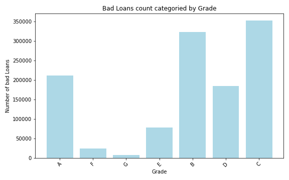
    %spark.pyspark
    # Create the Spark DataFrame
    loanGrade = filtered_df.filter(col('loan_status') != 'Good Loan') \
                 .groupBy('grade') \
                 .count() \
                 .withColumnRenamed('count', 'bad_laon_count')
    # Convert to pandas
    loanPan = loanGrade.toPandas()

    plt.figure(figsize=(8, 5))
    plt.bar(loanPan['grade'], loanPan['bad_laon_count'], color='lightblue')
    plt.title('Bad Loans count categoried by Grade')
    plt.xlabel('Grade')
    plt.ylabel('Number of bad Loans')
    plt.xticks(rotation=45)
    plt.tight_layout()
    plt.show()
Output:

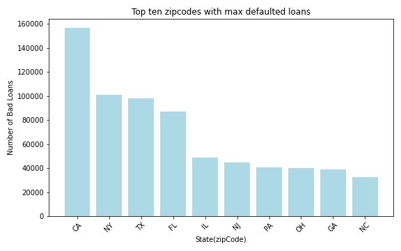
    %spark.pyspark
    loanAmtDF = filtered_df.filter(col('loan_status') != 'Good Loan') \
                  .groupBy('addr_state') \
                  .agg(count('*').alias('loanCount')) \
                  .withColumnRenamed('addr_state', 'State(zipCode)') \
                  .orderBy(desc('loanCount')) \
                  .limit(10)

    AmtDFPan = loanAmtDF.toPandas()

    plt.figure(figsize=(8, 5))
    plt.bar(AmtDFPan['State(zipCode)'], AmtDFPan['loanCount'], color='lightblue')
    plt.title('Top ten zipcodes with max defaulted loans')
    plt.xlabel('State(zipCode)')
    plt.ylabel('Number of Bad Loans')
    plt.xticks(rotation=45)
    plt.tight_layout()
    plt.show()
Output:
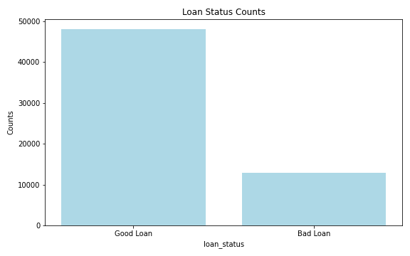
    %spark.pyspark
    loanStat = filtered_df.groupBy('loan_status') \
      .count() \
      .filter(col('loan_status').isin('Good Loan','Bad Loan'))

    # Convert to pandas
    loanStatPan = loanStat.toPandas()

    plt.figure(figsize=(8, 5))
    plt.bar(loanStatPan['loan_status'], loanStatPan['count'], color='lightblue')
    plt.title('Loan Status Counts')
    plt.xlabel('loan_status')
    plt.ylabel('Counts')
    plt.tight_layout()
    plt.show()
Output:
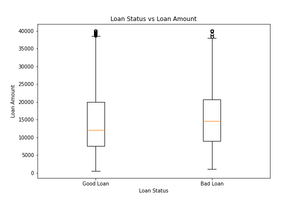
    %spark.pyspark
    pdf = filtered_df.select("loan_amnt", "loan_status").toPandas()

    plt.boxplot([
        pdf[pdf.loan_status=="Good Loan"].loan_amnt,
        pdf[pdf.loan_status=="Bad Loan"].loan_amnt
    ], labels=["Good Loan", "Bad Loan"])

    plt.title("Loan Status vs Loan Amount")
    plt.xlabel("Loan Status")
    plt.ylabel("Loan Amount")
    plt.show()
Output:
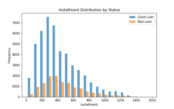
    %spark.pyspark
    # Convert to Pandas for plotting
    pandas_df = filtered_df.select('installment', 'loan_status').toPandas()
    fig, ax = plt.subplots(figsize=(8, 5))

    # Installment - Histograms
    good_loan_inst = pandas_df[pandas_df['loan_status'] == 'Good Loan']['installment']
    bad_loan_inst = pandas_df[pandas_df['loan_status'] == 'Bad Loan']['installment']

    ax.hist([good_loan_inst, bad_loan_inst], bins=20, label=['Good Loan', 'Bad Loan'], alpha=0.7)
    ax.set_title('Installment Distribution by Status')
    ax.set_xlabel('Installment')
    ax.set_ylabel('Frequency')
    ax.legend()
Output:
6. Feature engineering, transformation and data preparation for modeling.
StringIndexer to convert ‘grade’ column into numerical indices
    %spark.pyspark
    grade_indexer = StringIndexer(inputCol="grade", outputCol="grade_index", stringOrderType="alphabetAsc")

    df = grade_indexer\
    .fit(df)\
    .transform(df)\
    .drop('grade')
Functions
    %spark.pyspark
    def one_hot_encode_column(df, input_col):
        indexer = StringIndexer(inputCol=input_col, outputCol=input_col + '_indexed')
        indexed_df = indexer.fit(df).transform(df)

        encoder = OneHotEncoder(inputCol=input_col + '_indexed', outputCol=input_col + '_encoded')
        encoded_df = encoder.fit(indexed_df).transform(indexed_df)

        encoded_df = encoded_df.drop(input_col, input_col + '_indexed')

        return encoded_df
One Hot Encoder
    %spark.pyspark
    columns_to_encode = ['purpose', 'addr_state', 'home_ownership', 'initial_list_status']

    for column in columns_to_encode:
        df = one_hot_encode_column(df, column)
Cast to float type
    %spark.pyspark
    columns_to_cast = [ 'installment',
                       'int_rate',
                        'loan_amnt',
                        'annual_inc',
                        'dti',
                        'tax_liens',
                        'delinq_amnt',
                        'policy_code',
                        'last_fico_range_high',
                        'last_fico_range_low',
                        'recoveries',
                        'collection_recovery_fee'
    ]

    # cast to float
    for column_name in columns_to_cast:
        df = df.withColumn(column_name, col(column_name).cast('float'))
    %spark.pyspark
    df.printSchema()
Output:
    root
     |-- id: string (nullable = true)
     |-- term: integer (nullable = true)
     |-- acc_now_delinq: integer (nullable = true)
     |-- annual_inc: float (nullable = true)
     |-- application_type: integer (nullable = true)
     |-- dti: float (nullable = true)
     |-- installment: float (nullable = true)
     |-- int_rate: float (nullable = true)
     |-- loan_amnt: float (nullable = true)
     |-- loan_status: string (nullable = true)
     |-- tax_liens: float (nullable = true)
     |-- delinq_amnt: float (nullable = true)
     |-- policy_code: float (nullable = true)
     |-- last_fico_range_high: float (nullable = true)
     |-- last_fico_range_low: float (nullable = true)
     |-- recoveries: float (nullable = true)
     |-- collection_recovery_fee: float (nullable = true)
     |-- verification_status_encoded: integer (nullable = false)
     |-- grade_index: double (nullable = false)
     |-- purpose_encoded: vector (nullable = true)
     |-- addr_state_encoded: vector (nullable = true)
     |-- home_ownership_encoded: vector (nullable = true)
     |-- initial_list_status_encoded: vector (nullable = true)
Counting data according to loan_status.
    %spark.pyspark
    df.groupby('loan_status').count()\
    .show()
Output:
    +--------------------+-------+
    |         loan_status|  count|
    +--------------------+-------+
    |          Fully Paid|1076218|
    |             Default|     40|
    |  Late (31-120 days)|  21443|
    |             Current| 877018|
    |     In Grace Period|   8427|
    |Does not meet the...|    741|
    |Does not meet the...|   1913|
    |         Charged Off| 268452|
    |   Late (16-30 days)|   4344|
    +--------------------+-------+
Droping current rows
    %spark.pyspark
    df = df.filter(df.loan_status != 'Current')

    df.groupby('loan_status').count()\
    .show()
Output:
    +--------------------+-------+
    |         loan_status|  count|
    +--------------------+-------+
    |          Fully Paid|1076218|
    |             Default|     40|
    |  Late (31-120 days)|  21443|
    |     In Grace Period|   8427|
    |Does not meet the...|    741|
    |Does not meet the...|   1913|
    |         Charged Off| 268452|
    |   Late (16-30 days)|   4344|
    +--------------------+-------+
Encode ‘loan_status’ to 0 & 1, rename ‘loan_status’ to target and cast to Int.
    %spark.pyspark
    df = df.withColumn(
        "target",
        when(col("loan_status") == "Fully Paid", 0)
        .when(
            (col("loan_status").isin("In Grace Period")), 0)
        .when(
            col("loan_status") == "Does not meet the credit policy. Status:Fully Paid", 0)
        .when(
            col("loan_status").isin(
                "Does not meet the credit policy. Status:Charged Off",
                "Charged Off",
                "Late (16-30 days)",
                "Late (31-120 days)",
                "Default"
            ), 1)
        .otherwise(None))\
        .drop("loan_status")

    # Filter out rows where 'target' is null and cast 'target' to int
    df = df.filter(col("target").isNotNull()) \
        .withColumn("target", col("target").cast("int"))
    %spark.pyspark
    df.groupby('target').count()\
     .show()
Output:
    +------+-------+
    |target|  count|
    +------+-------+
    |     1| 295020|
    |     0|1086558|
    +------+-------+
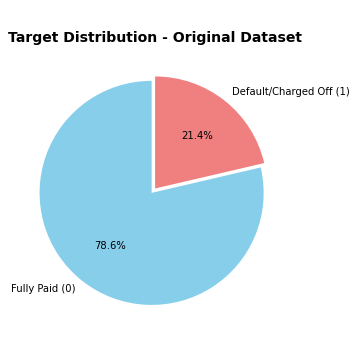
    %spark.pyspark
    counts = [1086558, 295020]
    labels = ['Fully Paid (0)', 'Default/Charged Off (1)']
    colors = ['skyblue', 'lightcoral']

    # Plot
    plt.figure(figsize=(5, 5))
    plt.pie(
        counts,
        labels=labels,
        autopct='%1.1f%%',
        startangle=90,
        colors=colors,
        explode=(0.05, 0)  # slight separation for clarity
    )
    plt.title('Target Distribution - Original Dataset', fontsize=14, fontweight='bold')
    plt.tight_layout()
    plt.show()
Output:
Droping id
    %spark.pyspark
    df = df.drop('id')
    df.show(3)
Output:
    +----+--------------+----------+----------------+-----+-----------+--------+---------+---------+-----------+-----------+--------------------+-------------------+----------+-----------------------+---------------------------+-----------+---------------+------------------+----------------------+---------------------------+------+
    |term|acc_now_delinq|annual_inc|application_type|  dti|installment|int_rate|loan_amnt|tax_liens|delinq_amnt|policy_code|last_fico_range_high|last_fico_range_low|recoveries|collection_recovery_fee|verification_status_encoded|grade_index|purpose_encoded|addr_state_encoded|home_ownership_encoded|initial_list_status_encoded|target|
    +----+--------------+----------+----------------+-----+-----------+--------+---------+---------+-----------+-----------+--------------------+-------------------+----------+-----------------------+---------------------------+-----------+---------------+------------------+----------------------+---------------------------+------+
    |  36|             0|   55000.0|               1| 5.91|     123.03|   13.99|   3600.0|      0.0|        0.0|        1.0|               564.0|              560.0|       0.0|                    0.0|                          1|        2.0| (13,[0],[1.0])|    (50,[6],[1.0])|         (5,[0],[1.0])|              (1,[0],[1.0])|     0|
    |  36|             0|   65000.0|               1|16.06|     820.28|   11.99|  24700.0|      0.0|        0.0|        1.0|               699.0|              695.0|       0.0|                    0.0|                          1|        2.0| (13,[6],[1.0])|   (50,[47],[1.0])|         (5,[0],[1.0])|              (1,[0],[1.0])|     0|
    |  60|             0|   63000.0|               0|10.78|     432.66|   10.78|  20000.0|      0.0|        0.0|        1.0|               704.0|              700.0|       0.0|                    0.0|                          1|        1.0| (13,[2],[1.0])|    (50,[4],[1.0])|         (5,[0],[1.0])|              (1,[0],[1.0])|     0|
    +----+--------------+----------+----------------+-----+-----------+--------+---------+---------+-----------+-----------+--------------------+-------------------+----------+-----------------------+---------------------------+-----------+---------------+------------------+----------------------+---------------------------+------+
    only showing top 3 rows
Split the data into training and test sets (20% held out for testing)
    %spark.pyspark

    train_df, test_df = df.randomSplit([0.8, 0.2], seed=42)

    print(f"\nTraining set: {train_df.count()} rows")
    print(f"Test set: {test_df.count()} rows")
Output:
    Training set: 1105548 rows
    Test set: 276030 rows
VectorAssembler and MinMaxScaler
    %spark.pyspark
    all_columns = df.columns
    feature_columns = [col_name for col_name in all_columns if col_name != 'target']

    # Create data preparation pipeline stages
    assembler = VectorAssembler(inputCols=feature_columns, outputCol="rawFeatures")
    scaler = MinMaxScaler(inputCol="rawFeatures", outputCol="features")
7. Classification
DecisionTreeClassifer
    %spark.pyspark
    # Train a DecisionTree model
    dt = DecisionTreeClassifier(labelCol="target", featuresCol="features")

    # Chain indexers, assembler, scaler and tree in a Pipeline
    dt_pipeline = Pipeline(stages=[assembler, scaler, dt])
    %spark.pyspark
    # Train model. This also runs the indexers, assembler and scaler.
    dt_model = dt_pipeline.fit(train_df)

    # Make predictions.
    dt_predictions = dt_model.transform(test_df)

    # Select example rows to display.
    dt_predictions.select("prediction", "target", "features").show(5)
Output:
    +----------+------+--------------------+
    |prediction|target|            features|
    +----------+------+--------------------+
    |       0.0|     1|(86,[2,4,5,6,7,10...|
    |       0.0|     0|(86,[2,4,5,6,7,10...|
    |       1.0|     1|(86,[2,4,5,6,7,10...|
    |       0.0|     1|(86,[2,4,5,6,7,10...|
    |       0.0|     0|(86,[2,4,5,6,7,10...|
    +----------+------+--------------------+
    only showing top 5 rows
    %spark.pyspark
    # Select (prediction, true label) and compute test error

    dt_evaluator = MulticlassClassificationEvaluator(
        labelCol="target",
        predictionCol="prediction"
    )

    dt_accuracy = dt_evaluator.evaluate(dt_predictions, {dt_evaluator.metricName: "accuracy"})
    dt_f1 = dt_evaluator.evaluate(dt_predictions, {dt_evaluator.metricName: "f1"})

    # Calculate additional metrics using MulticlassMetrics
    dt_prediction_and_labels = dt_predictions.select("prediction", "target").rdd.map(
        lambda row: (float(row['prediction']), float(row['target']))
    )
    dt_metrics = MulticlassMetrics(dt_prediction_and_labels)

    dt_precision = dt_metrics.precision(1.0)
    dt_recall = dt_metrics.recall(1.0)

    # print(f"Test Accuracy = {accuracy:.4f}")

    print("Decision tree Evaluation Metrics:")
    print(f"Accuracy: {dt_accuracy:.4f}")
    print(f"F1-Score: {dt_f1:.4f}")
    print(f"Precision (Class 1): {dt_precision:.4f}")
    print(f"Recall (Class 1): {dt_recall:.4f}")

    # Show confusion matrix
    print("Confusion Matrix:")
    print(dt_metrics.confusionMatrix().toArray())
Output:
    Decision tree Evaluation Metrics:
    Accuracy: 0.9381
    F1-Score: 0.9355
    Precision (Class 1): 0.9429
    Recall (Class 1): 0.7557
    Confusion Matrix:
    [[214443.   2696.]
     [ 14389.  44502.]]
RandomForestClassifier
    %spark.pyspark
    # Train a RandomForest model.
    rf = RandomForestClassifier(
        labelCol="target",
        featuresCol="features",
        numTrees=100,
        seed=42,
        maxDepth=10
    )

    # Chain assembler, scaler and forest in a Pipeline
    rf_pipeline = Pipeline(stages=[assembler, scaler, rf])
    %spark.pyspark
    # Train model. This also runs the assembler and scaler.
    rf_model = rf_pipeline.fit(train_df)

    # Make predictions.
    rf_predictions = rf_model.transform(test_df)

    # Select example rows to display.
    print("Sample predictions:")
    rf_predictions.select("prediction", "target", "probability", "features").show(5)
Output:
    Sample predictions:
    +----------+------+--------------------+--------------------+
    |prediction|target|         probability|            features|
    +----------+------+--------------------+--------------------+
    |       0.0|     1|[0.95210802562047...|(86,[2,4,5,6,7,10...|
    |       0.0|     0|[0.95633576378056...|(86,[2,4,5,6,7,10...|
    |       1.0|     1|[0.02718347317466...|(86,[2,4,5,6,7,10...|
    |       1.0|     1|[0.43039329849675...|(86,[2,4,5,6,7,10...|
    |       0.0|     0|[0.93486641199661...|(86,[2,4,5,6,7,10...|
    +----------+------+--------------------+--------------------+
    only showing top 5 rows
    %spark.pyspark
    # Evaluate the model
    rf_evaluator = MulticlassClassificationEvaluator(
        labelCol="target",
        predictionCol="prediction"
    )

    # Calculate multiple metrics
    rf_accuracy = rf_evaluator.evaluate(rf_predictions, {rf_evaluator.metricName: "accuracy"})
    rf_f1 = rf_evaluator.evaluate(rf_predictions, {rf_evaluator.metricName: "f1"})
    rf_weighted_precision = rf_evaluator.evaluate(rf_predictions, {rf_evaluator.metricName: "weightedPrecision"})
    rf_weighted_recall = rf_evaluator.evaluate(rf_predictions, {rf_evaluator.metricName: "weightedRecall"})

    print("\nRandomForest Evaluation Metrics:")
    print(f"Accuracy: {rf_accuracy:.4f}")
    print(f"F1-Score: {rf_f1:.4f}")
    print(f"Weighted Precision: {rf_weighted_precision:.4f}")
    print(f"Weighted Recall: {rf_weighted_recall:.4f}")

    # Confusion Matrix
    print("\nConfusion Matrix:")
    rf_prediction_and_labels = rf_predictions.select("prediction", "target").rdd.map(
        lambda row: (float(row['prediction']), float(row['target']))
    )
    rf_metrics = MulticlassMetrics(rf_prediction_and_labels)
    print(rf_metrics.confusionMatrix().toArray())
Output:
    RandomForest Evaluation Metrics:
    Accuracy: 0.9408
    F1-Score: 0.9387
    Weighted Precision: 0.9406
    Weighted Recall: 0.9408

    Confusion Matrix:
    [[214016.   3123.]
     [ 13216.  45675.]]
SparkXGBClassifier
    %spark.pyspark

    xgb = SparkXGBClassifier(
        features_col="features",
        label_col="target",
        num_workers=2,
        eval_metric="logloss",
        eta=0.1,
        max_depth=5,
        num_round=10
    )


    # Chain assembler, scaler and XGBoost in a Pipeline
    xgb_pipeline = Pipeline(stages=[assembler, scaler, xgb])
    %spark.pyspark
    # Train model with timing
    print("Training XGBoost model...")

    xgb_model = xgb_pipeline.fit(train_df)

    # Make predictions
    print("Making predictions...")
    xgb_predictions = xgb_model.transform(test_df)

    # Select example rows to display
    print("\nSample predictions:")
    xgb_predictions.select("prediction", "target", "probability", "rawPrediction", "features").show(5, truncate=False)
Output:
    Training XGBoost model...
    2025-10-29 20:47:21,734 INFO XGBoost-PySpark: _fit Running xgboost-3.1.0 on 2 workers with
	    booster params: {'objective': 'binary:logistic', 'device': 'cpu', 'eval_metric': 'logloss', 'max_depth': 5, 'eta': 0.1, 'num_round': 10, 'nthread': 1}
	    train_call_kwargs_params: {'verbose_eval': True, 'num_boost_round': 100}
	    dmatrix_kwargs: {'nthread': 1, 'missing': nan}
    2025-10-29 20:49:52,939 INFO XGBoost-PySpark: _fit Finished xgboost training!
    Making predictions...

    Sample predictions:
    +----------+------+------------------------------------------+----------------------------------------+---------------------------------------------------------------------------------------------------------------------------------------------------------------------------------------------------------------------------------------------------------------+
    |prediction|target|probability                               |rawPrediction                           |features                                                                                                                                                                                                                                                       |
    +----------+------+------------------------------------------+----------------------------------------+---------------------------------------------------------------------------------------------------------------------------------------------------------------------------------------------------------------------------------------------------------------+
    |0.0       |1     |[0.9660659432411194,0.03393407166004181]  |[3.3488125801086426,-3.3488125801086426]|(86,[2,4,5,6,7,10,11,12,15,16,18,79,80,85],[1.4546533633767742E-6,1.0,0.3809435178841951,0.18574766405031984,0.5031645569620253,0.5,0.9458823529411764,0.9467455621301776,1.0,0.16666666666666666,1.0,1.0,1.0,1.0])                                            |
    |0.0       |0     |[0.9153358936309814,0.08466409891843796]  |[2.3805994987487793,-2.3805994987487793]|(86,[2,4,5,6,7,10,11,12,18,31,80,85],[5.3094847763252255E-5,0.039,0.10554551138116217,0.07515575705763099,0.13924050632911394,0.5,0.828235294117647,0.8284023668639053,1.0,1.0,1.0,1.0])                                                                       |
    |1.0       |1     |[1.8674135208129883E-4,0.9998132586479187]|[-8.585590362548828,8.585590362548828]  |(86,[2,4,5,6,7,10,11,12,13,14,15,16,17,30,81,85],[5.3094847763252255E-5,1.0,0.6954632845468051,0.3415109049669293,0.8734177215189874,0.5,0.6399999999999999,0.6390532544378699,0.09259622605372142,0.09388948490933186,1.0,0.3333333333333333,1.0,1.0,1.0,1.0])|
    |1.0       |1     |[0.13452231884002686,0.8654776811599731]  |[-1.861551284790039,1.861551284790039]  |(86,[2,4,5,6,7,10,11,12,15,16,26,30,81,85],[8.47335584166971E-5,1.0,0.050177856274455035,0.6285047090362108,0.04810126582278481,0.5,0.6458823529411765,0.6449704142011834,1.0,0.5,1.0,1.0,1.0,1.0])                                                            |
    |0.0       |0     |[0.9195100665092468,0.08048991858959198]  |[2.435708999633789,-2.435708999633789]  |(86,[2,4,5,6,7,10,11,12,15,16,18,30,81,85],[8.946118184767161E-5,0.8190999755859375,0.6532859226592638,0.1728971996456476,0.8734177215189874,0.5,0.8870588235294117,0.8875739644970414,1.0,0.16666666666666666,1.0,1.0,1.0,1.0])                               |
    +----------+------+------------------------------------------+----------------------------------------+---------------------------------------------------------------------------------------------------------------------------------------------------------------------------------------------------------------------------------------------------------------+
    only showing top 5 rows
    %spark.pyspark
    # Evaluate the model
    xgb_evaluator = MulticlassClassificationEvaluator(
        labelCol="target",
        predictionCol="prediction"
    )

    # Calculate multiple metrics
    xgb_accuracy = xgb_evaluator.evaluate(xgb_predictions, {xgb_evaluator.metricName: "accuracy"})
    xgb_f1 = xgb_evaluator.evaluate(xgb_predictions, {xgb_evaluator.metricName: "f1"})
    xgb_weighted_precision = xgb_evaluator.evaluate(xgb_predictions, {xgb_evaluator.metricName: "weightedPrecision"})
    xgb_weighted_recall = xgb_evaluator.evaluate(xgb_predictions, {xgb_evaluator.metricName: "weightedRecall"})


    print("XGBOOST EVALUATION METRICS")
    print(f"Accuracy: {xgb_accuracy:.4f}")
    print(f"F1-Score: {xgb_f1:.4f}")
    print(f"Weighted Precision: {xgb_weighted_precision:.4f}")
    print(f"Weighted Recall: {xgb_weighted_recall:.4f}")

    # Confusion Matrix
    print("CONFUSION MATRIX")

    xgb_prediction_and_labels = xgb_predictions.select("prediction", "target").rdd.map(
        lambda row: (float(row['prediction']), float(row['target']))
    )
    xgb_metrics = MulticlassMetrics(xgb_prediction_and_labels)
    xgb_conf_matrix = xgb_metrics.confusionMatrix().toArray()
    print(xgb_conf_matrix)
Output:
    XGBOOST EVALUATION METRICS
    Accuracy: 0.9457
    F1-Score: 0.9445
    Weighted Precision: 0.9449
    Weighted Recall: 0.9457
    CONFUSION MATRIX
    [[212945.   4194.]
     [ 10799.  48092.]]
Analysis of Classifier Results.
The models using a single train-test split, such as an 80/20 division. The reported metrics are:
| Model | Accuray | F1-Score | Precision | Recall |
|---|---|---|---|---|
| Decision Tree | 0.9381 | 0.9355 | 0.9429 | 0.7557 |
| Random Forest | 0.9408 | 0.9387 | 0.9406 | 0.9408 |
| XGBoost | 0.9457 | 0.9445 | 0.9449 | 0.9457 |
Observation:
- The Decision Tree shows lower recall → it misses more positive cases.
- Random Forest and XGBoost generalize better, but their gains are marginal (≈0.3–0.5%).
- The performance differences may not be statistically significant without testing on multiple splits.
XGBoost Cross-Validation
    %spark.pyspark
    paramGrid = (
        ParamGridBuilder()
        .addGrid(xgb.max_depth, [4, 5])
        .addGrid(xgb.arbitrary_params_dict, [
            {"eta": 0.1, "num_round": 10},
            {"eta": 0.2, "num_round": 10}
        ])
        .build()
    )

    # Evaluator
    evaluator = MulticlassClassificationEvaluator(
        labelCol="target", predictionCol="prediction", metricName="f1"
    )


    cv = CrossValidator(
        estimator=xgb_pipeline,
        estimatorParamMaps=paramGrid,
        evaluator=evaluator,
        numFolds=2,
        parallelism=1,
        seed=42
    )
    start_time = time.time()
    print("Running Lightweight XGBoost Cross-Validation...")

    cv_model = cv.fit(train_df)

    print(f"CV completed in {(time.time() - start_time)/60:.2f} minutes")

    best_model = cv_model.bestModel
    best_xgb = best_model.stages[-1]

    print("\n=== Best Parameters ===")
    print("max_depth:", best_xgb.getOrDefault("max_depth"))
    print("arbitrary_params_dict:", best_xgb.getOrDefault("arbitrary_params_dict"))
Output:
    Running Lightweight XGBoost Cross-Validation...
    2025-10-29 21:02:24,001 INFO XGBoost-PySpark: _fit Running xgboost-3.1.0 on 2 workers with
	    booster params: {'device': 'cpu', 'eval_metric': 'logloss', 'max_depth': 4, 'objective': 'binary:logistic', 'eta': 0.1, 'num_round': 10, 'nthread': 1}
	    train_call_kwargs_params: {'verbose_eval': True, 'num_boost_round': 100}
	    dmatrix_kwargs: {'nthread': 1, 'missing': nan}
    2025-10-29 21:02:48,290 INFO XGBoost-PySpark: _fit Finished xgboost training!
    2025-10-29 21:04:44,629 INFO XGBoost-PySpark: _fit Running xgboost-3.1.0 on 2 workers with
	    booster params: {'device': 'cpu', 'eval_metric': 'logloss', 'max_depth': 4, 'objective': 'binary:logistic', 'eta': 0.2, 'num_round': 10, 'nthread': 1}
	    train_call_kwargs_params: {'verbose_eval': True, 'num_boost_round': 100}
	    dmatrix_kwargs: {'nthread': 1, 'missing': nan}
                    .
                    .
                    .
    CV completed in 20.21 minutes

    === Best Parameters ===
    max_depth: 5
    arbitrary_params_dict: {'eta': 0.2, 'num_round': 10}
    %spark.pyspark
    print("Evaluating best model on test set...")

    best_predictions = best_model.transform(test_df)

    # Evaluate multiple metrics
    metrics = {}
    for metric in ["accuracy", "f1", "weightedPrecision", "weightedRecall"]:
        metrics[metric] = evaluator.evaluate(best_predictions, {evaluator.metricName: metric})

    print("\nXGBOOST CROSS-VALIDATED TEST RESULTS")
    for m, v in metrics.items():
        print(f"{m.capitalize():<20}: {v:.4f}")

    # Confusion Matrix
    from pyspark.mllib.evaluation import MulticlassMetrics

    preds_and_labels=best_predictions.select("prediction", "target" ).rdd.map(
    lambda row: (float(row['prediction']), float(row['target'])))

    metrics_obj=MulticlassMetrics(preds_and_labels)
    conf_matrix=metrics_obj.confusionMatrix().toArray()

    print("\nCONFUSION MATRIX")
    print(conf_matrix)
Output:
    Evaluating best model on test set...

    XGBOOST CROSS-VALIDATED TEST RESULTS
    Accuracy            : 0.9485
    F1                  : 0.9475
    Weightedprecision   : 0.9478
    Weightedrecall      : 0.9485

    CONFUSION MATRIX
    [[213082.   4057.]
     [ 10148.  48743.]]
These results clearly show that cross-validation improved our XGBoost model’s generalization. Let’s analyze them carefully and discuss what this improvement means and why cross-validation was beneficial in our case.
Comparison Summary
| Metric | Before CV | After CV | Change | Interpretation |
|---|---|---|---|---|
| Accuracy | 0.9457 | 0.9485 | ↑ +0.0028 | Better prediction consistency |
| F1-Score | 0.9445 | 0.9475 | ↑ +0.0030 | Improved precision-recall balance |
| Weighted Precision | 0.9449 | 0.9478 | ↑ +0.0029 | More reliable positive predictions |
| Weighted Recall | 0.9457 | 0.9485 | ↑ +0.0028 | Capturing slightly more true positives |
| False Positives(FP) | 4194 | 4057 | ↓ -137 | Fewer incorrect positive predictions |
| False Negatives(FN) | 10799 | 10148 | ↓ -651 | Model is missing fewer positive cases |
Overall, both types of classification errors decreased, showing the model is better tuned and generalizes more effectively.
Technical Insight
Cross-validation averages performance across folds:
\[\text{Cross-Validation Accuracy}=\frac{1}{k}\sum _{i=1}^{k}\text{Accuracy}_{i}\]
So, even small improvements (like +0.0028) are statistically meaningful in large datasets — our test set has over 270K samples, meaning thousands of extra correct predictions.
Final Interpretation
Cross-validation improved:
- Accuracy by 0.28%
- F1 by 0.30%,
- Reduced 788 total errors(FP + FN combined).
Model Evaluation and the Effect of Cross-Validation
The initial XGBoost model demonstrated strong predictive capability, achieving an accuracy of 94.57%
and an F1-score of 94.45% on the test set. However, following the application of k-fold cross-validation
with hyperparameter optimization, the model’s performance improved further, reaching an accuracy of 94.85%
and an F1-score of 94.75%. This enhancement indicates that cross-validation effectively reduced variance
and improved model generalization by ensuring that each data subset contributed to both training and
validation processes. The resulting model exhibited a more balanced classification performance, with
reduced false positives and false negatives, demonstrating the importance of cross-validation in
developing a stable and reliable predictive framework for large-scale data analysis tasks.
8. References

Image:freepik