Running Logistic regression and Linear regression on Hadoop Cluster using Apache Spark's Scala API
In this article, we will explore supervised machine learning using Scala, leveraging Spark’s
scalable ML libraries on a Hadoop cluster. This project outlines the development of predictive
regression models using a modern big data stack We will leverage the scalability
of Hadoop 3.3.0 for distributed storage and the high-performance processing engine of
Spark 3.1.1 for in-memory analytics. Our goal is to build and evaluate both a Logistic
Regression classifier and a Linear Regression model using a classic dataset:
the yellow_tripdata_2014-08.csv file, which contains records of New York City
yellow taxi trips for August 2014.

Nature photo created by wirestock - www.freepik.com
If you are interested with the data you can collect it from here Click the link. 2014 Yellow NYC taxi trip Data . For Classification method, our task is to implement a model to predict for a given taxi trip, if a tip will be paid or not for a trip. And for Regression method, our task is to implement a model to predict for a given taxi trip, what is the expected tip amount for a trip. Hadoop environment is three nodes cluster, one namenode and two datanodes.
Here we will use Scala 2.12.10 version and IntelliJ IDEA edition 2020.3 for this module. Our essential sbt dependency commands of build.sbt are as following
        name := "ScalaNycTaxi"
        version := "0.1"
        scalaVersion := "2.12.10"

        libraryDependencies ++= Seq(
          "org.apache.spark" %% "spark-core" % "3.1.1",
          "org.apache.spark" %% "spark-sql" % "3.1.1",
          "org.apache.spark" %% "spark-mllib" % "3.1.1",
          "org.scalanlp" %% "breeze-viz" % "1.1"
        )
Import libraries
The Spark, ML, and other libraries we'll need by using the following lines of code
        import breeze.plot.{Figure, plot}
        import org.apache.spark.ml.classification.LogisticRegression
        import org.apache.spark.ml.evaluation.{BinaryClassificationEvaluator, MulticlassClassificationEvaluator, RegressionEvaluator}
        import org.apache.spark.ml.feature.{OneHotEncoder, StringIndexer, VectorAssembler}
        import org.apache.spark.ml.linalg.DenseVector
        import org.apache.spark.ml.regression.LinearRegression
        import org.apache.spark.mllib.evaluation.BinaryClassificationMetrics
        import org.apache.spark.sql.functions.col
        import org.apache.spark.sql.{Row, SparkSession}
        import org.apache.spark.sql.types.{DoubleType, StringType, StructField, StructType}
        import breeze.stats.hist._
        import org.apache.spark.sql.functions._
        import breeze.linalg.{DenseVector => BDenseVector}
Data Exploration
At first we ingest the data that we want to analyze. The data is brought from external sources or systems where it resides into data exploration and modeling environment. The data exploration and modeling environment is Spark. Firstly we need to make sure our source of data that is our dataset files are present in HDFS where we expect to read them from our spark jobs. To put the files in HDFS first bring the files to the operating system i.e. Linux in our case and from Linux we copy them to HDFS using the following command
We will first load dataset using Apache Spark and see the total numbers of rows, header, and first 5 rows of our dataset. For these our lines of codes are shown bellow
            val spark = SparkSession.builder()
                  .master("local[*]")
                  .appName("SparkByExamples.com")
                  .getOrCreate();
            val dataRaw = spark.sparkContext
                    .textFile("hdfs://master:9000/data/data/yellow_tripdata_2014-08.csv")
            val header = dataRaw.first();
Now we print the header of the dataset.
println(header);
Output:
vendor_id, pickup_datetime, dropoff_datetime, passenger_count, trip_distance, pickup_longitude, pickup_latitude, rate_code, store_and_fwd_flag, dropoff_longitude, dropoff_latitude, payment_type, fare_amount, surcharge, mta_tax, tip_amount, tolls_amount, total_amount
Total numbers of records of Dataset
println("Total Records : " + dataRaw.count());
Output:
Total Records : 12688879
The code of first 5 rows of the dataset is as follows
dataRaw.take(5).foreach(x => println(x))
OutPut:
        vendor_id, pickup_datetime, dropoff_datetime, passenger_count, trip_distance, pickup_longitude, pickup_latitude, rate_code, store_and_fwd_flag, dropoff_longitude, dropoff_latitude, payment_type, fare_amount, surcharge, mta_tax, tip_amount, tolls_amount, total_amount

        CMT,2014-08-16 14:58:49,2014-08-16 15:15:59,1,2.7000000000000002,-73.946537000000006,40.776812999999997,1,N,-73.976192999999995,40.755625000000002,CSH,14,0,0.5,0,0,14.5
        CMT,2014-08-16 08:10:48,2014-08-16 08:58:16,3,20.399999999999999,-73.776857000000007,40.645099000000002,1,Y,-73.916248999999993,40.837356999999997,CSH,58.5,0,0.5,0,5.3300000000000001,64.329999999999998
        CMT,2014-08-16 09:44:07,2014-08-16 09:54:37,1,2.1000000000000001,-73.986585000000005,40.725847999999999,1,N,-73.977157000000005,40.751961000000001,CSH,9.5,0,0.5,0,0,10
Now we can see the dataset rows printed above, We loaded the dataset from an HDFS location and stored it in an RDD of strings. Fortunately, the dataset is relatively clean and has one row per data item but it contains a empty row. Next, we remove the header, delete the empty row and again print 5 rows from the dataset, we run the codes following
        val dataLines = dataRaw.filter(r => !r.isEmpty)
            .filter(r => !r.startsWith("vendor_id"))

        dataLines.take(5).foreach(s => println(s))
Output:
        CMT,2014-08-16 14:58:49,2014-08-16 15:15:59,1,2.7000000000000002,-73.946537000000006,40.776812999999997,1,N,-73.976192999999995,40.755625000000002,CSH,14,0,0.5,0,0,14.5
        CMT,2014-08-16 08:10:48,2014-08-16 08:58:16,3,20.399999999999999,-73.776857000000007,40.645099000000002,1,Y,-73.916248999999993,40.837356999999997,CSH,58.5,0,0.5,0,5.3300000000000001,64.329999999999998
        CMT,2014-08-16 09:44:07,2014-08-16 09:54:37,1,2.1000000000000001,-73.986585000000005,40.725847999999999,1,N,-73.977157000000005,40.751961000000001,CSH,9.5,0,0.5,0,0,10
        CMT,2014-08-16 10:46:13,2014-08-16 10:51:25,1,1.3,-73.976290000000006,40.765231,1,N,-73.961484999999996,40.777889000000002,CSH,6,0,0.5,0,0,6.5
        CMT,2014-08-16 09:27:23,2014-08-16 09:39:37,2,1.7,-73.995248000000004,40.754646000000001,1,Y,-73.995902999999998,40.769201000000002,CSH,10.5,0,0.5,0,0,11
As seen, the rows of dataset are fine, now we generate schema based on the column strings of the header of the dataset, cast variables according to the schema, and create an initial dataframe and lastly see 10 rows of the dataset, for these we run the following codes
         val  schema = StructType(
              Array(
                StructField("vendor_id", StringType, true),
                StructField("pickup_datetime", StringType, true),
                StructField("dropoff_datetime", StringType, true),
                StructField("passenger_count", DoubleType, true),
                StructField("trip_distance", DoubleType, true),
                StructField("pickup_longitude", DoubleType, true),
                StructField("pickup_latitude", DoubleType, true),
                StructField("rate_code", DoubleType, true),
                StructField("store_and_fwd_flag", StringType, true),
                StructField("dropoff_longitude", DoubleType, true),
                StructField("dropoff_latitude", DoubleType, true),
                StructField("payment_type", StringType, true),
                StructField("fare_amount", DoubleType, true),
                StructField("surcharge", DoubleType, true),
                StructField("mta_tax", DoubleType, true),
                StructField("tip_amount", DoubleType, true),
                StructField("tolls_amount", DoubleType, true),
                StructField("total_amount", DoubleType, true)
              )
            )

        val rowRDD = dataLines
                .map(_.split(","))
                .map(p => Row(p(0), p(1), p(2), p(3).toDouble, p(4).toDouble, p(5).toDouble, p(6).toDouble,
                p(7).toDouble, p(8), p(9).toDouble, p(10).toDouble, p(11), p(12).toDouble, p(13).toDouble,
                p(14).toDouble, p(15).toDouble, p(16).toDouble, p(17).toDouble))

        val dataDF = spark.createDataFrame(rowRDD, schema)
        dataDF.show(10)
Output:
        +---------+-------------------+-------------------+---------------+-------------+----------------+---------------+---------+------------------+-----------------+----------------+------------+-----------+---------+-------+----------+------------+------------+
        |vendor_id|    pickup_datetime|   dropoff_datetime|passenger_count|trip_distance|pickup_longitude|pickup_latitude|rate_code|store_and_fwd_flag|dropoff_longitude|dropoff_latitude|payment_type|fare_amount|surcharge|mta_tax|tip_amount|tolls_amount|total_amount|
        +---------+-------------------+-------------------+---------------+-------------+----------------+---------------+---------+------------------+-----------------+----------------+------------+-----------+---------+-------+----------+------------+------------+
        |      CMT|2014-08-16 14:58:49|2014-08-16 15:15:59|            1.0|          2.7|      -73.946537|      40.776813|      1.0|                 N|       -73.976193|       40.755625|         CSH|       14.0|      0.0|    0.5|       0.0|         0.0|        14.5|
        |      CMT|2014-08-16 08:10:48|2014-08-16 08:58:16|            3.0|         20.4|      -73.776857|      40.645099|      1.0|                 Y|       -73.916249|       40.837357|         CSH|       58.5|      0.0|    0.5|       0.0|        5.33|       64.33|
        |      CMT|2014-08-16 09:44:07|2014-08-16 09:54:37|            1.0|          2.1|      -73.986585|      40.725848|      1.0|                 N|       -73.977157|       40.751961|         CSH|        9.5|      0.0|    0.5|       0.0|         0.0|        10.0|
        |      CMT|2014-08-16 10:46:13|2014-08-16 10:51:25|            1.0|          1.3|       -73.97629|      40.765231|      1.0|                 N|       -73.961485|       40.777889|         CSH|        6.0|      0.0|    0.5|       0.0|         0.0|         6.5|
        |      CMT|2014-08-16 09:27:23|2014-08-16 09:39:37|            2.0|          1.7|      -73.995248|      40.754646|      1.0|                 Y|       -73.995903|       40.769201|         CSH|       10.5|      0.0|    0.5|       0.0|         0.0|        11.0|
        |      CMT|2014-08-16 14:14:16|2014-08-16 14:25:33|            2.0|          1.7|      -73.991535|      40.759863|      1.0|                 N|       -74.005722|       40.737558|         CSH|       10.0|      0.0|    0.5|       0.0|         0.0|        10.5|
        |      CMT|2014-08-16 15:55:16|2014-08-16 16:00:10|            1.0|          1.0|      -73.972307|      40.794076|      1.0|                 N|       -73.963865|       40.807858|         CSH|        6.0|      0.0|    0.5|       0.0|         0.0|         6.5|
        |      CMT|2014-08-16 14:08:29|2014-08-16 14:32:03|            1.0|          9.2|      -73.967338|      40.766009|      1.0|                 N|       -73.872972|       40.774487|         CSH|       28.5|      0.0|    0.5|       0.0|         0.0|        29.0|
        |      CMT|2014-08-16 11:11:21|2014-08-16 11:23:48|            1.0|          2.6|      -73.973775|      40.794591|      1.0|                 N|       -73.970561|       40.768086|         CSH|       11.5|      0.0|    0.5|       0.0|         0.0|        12.0|
        |      CMT|2014-08-16 07:44:56|2014-08-16 07:49:26|            1.0|          1.4|       -73.98636|      40.737913|      1.0|                 N|       -73.977117|       40.751126|         CSH|        6.0|      0.0|    0.5|       0.0|         0.0|         6.5|
        +---------+-------------------+-------------------+---------------+-------------+----------------+---------------+---------+------------------+-----------------+----------------+------------+-----------+---------+-------+----------+------------+------------+
        only showing top 10 rows
We are not interested with all the columns of the dataset, we create a cleaned data frame by droping unwanted columns and filtering unwanted values, cache and materialize the data frame in memory, and register the cleaned data frame as a temporary table in sqlcontext.
        val dataDF_cleaned = dataDF
                .drop(dataDF.col("store_and_fwd_flag")).drop(dataDF.col("pickup_datetime"))
                .drop(dataDF.col("dropoff_datetime")).drop(dataDF.col("pickup_longitude"))
                .drop(dataDF.col("pickup_latitude")).drop(dataDF.col("dropoff_longitude"))
                .drop(dataDF.col("dropoff_latitude")).drop(dataDF.col("surcharge"))
                .drop(dataDF.col("mta_tax")).drop(dataDF.col("tolls_amount"))
                .drop(dataDF.col("total_amount"))
                .filter("passenger_count > 0 AND fare_amount >= 1 " +
                  "AND trip_distance > 0")

        dataDF_cleaned.cache()
        dataDF_cleaned.createOrReplaceTempView("tempView")
Data Visualization
In this section, we examine the data by using SQL queries and import the results into a data frame to plot the target variables and prospective features for visual inspection by using the automatic visualization. Here we are using Breeze-Viz 1.1 for graphical data representations.
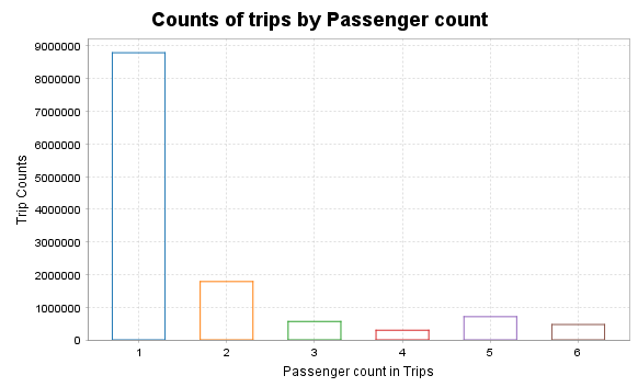
Counts of trips by passenger
        val plotDF1 = spark.sql("""
            SELECT passenger_count, COUNT(*) AS trip_counts
            FROM tempView
            WHERE passenger_count > 0 AND passenger_count < 7
            GROUP BY passenger_count
            ORDER BY passenger_count
        """)
        val rows = plotDF1.collect()

        val passengerCounts = rows.map(_.getAs[Double]("passenger_count"))
        val tripCounts = rows.map(_.getAs[Long]("trip_counts").toDouble)

        val fig = Figure()
        val plt = fig.subplot(0)

        val width = 0.6
        for (i <- passengerCounts.indices) {
                    val x=passengerCounts(i).toDouble
                    val y=tripCounts(i)
                    // Draw rectangle for each bar
                    plt +=plot(Seq(x - width /2, x - width /2, x + width /2, x + width /2, x - width /2),
                    Seq(0.0, y, y, 0.0, 0.0), '-' )
                    }
                    plt.title="Counts of trips by Passenger count"
                    plt.xlabel="Passenger count in Trips"
                    plt.ylabel="Trip Counts"
Output:

SQL Query and Data frame:
val plotDF2 = spark.sql("""
SELECT fare_amount, passenger_count, tip_amount
FROM tempView
WHERE passenger_count > 0 AND passenger_count < 7 AND
fare_amount > 0 AND fare_amount < 200 AND
payment_type in ('CSH', 'CRD') AND
tip_amount > 0 AND tip_amount < 25
LIMIT 10000
""")
val tipValues = plotDF2.select("tip_amount").collect().map(_.getDouble(0))
val fig = Figure()
val plt = fig.subplot(0)
val bins = 25
val minVal = tipValues.min
val maxVal = tipValues.max
val binWidth = (maxVal - minVal) / bins
val counts = Array.fill(bins)(0)
for (v <- tipValues) {
val idx=math.min(((v - minVal) / binWidth).toInt, bins - 1)
counts(idx) +=1
}
// Draw bars manually
for (i <- 0 until bins) {
val xLeft = minVal + i * binWidth
val xRight = xLeft + binWidth
val yTop = counts(i).toDouble
val xs = BDenseVector(Array(xLeft, xRight, xRight, xLeft, xLeft))
val ys = BDenseVector(Array(0.0, 0.0, yTop, yTop, 0.0))
plt += plot(xs, ys, name = "tip_amount")
}
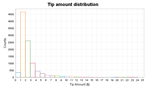
plt.title = "Tip amount distribution"
plt.xlabel = "Tip Amount ($)"
plt.ylabel = "Counts"
Histogram of tip amount
Output:
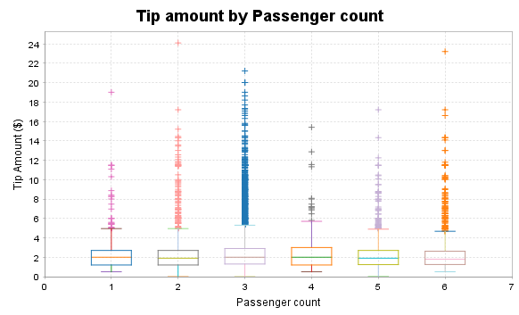
Relationship between tip amount and Passenger Count
        val plotDF2 = spark.sql("""
          SELECT fare_amount, passenger_count, tip_amount
          FROM tempView
          WHERE passenger_count > 0 AND passenger_count < 7 AND
                fare_amount > 0 AND fare_amount < 200 AND
                payment_type in ('CSH', 'CRD') AND
                tip_amount > 0 AND tip_amount < 25
          LIMIT 10000
        """)

        val grouped = plotDF2.groupBy("passenger_count")
          .agg(collect_list("tip_amount").alias("tips"))
          .collect()

        val passengerGroups = grouped.map(row => row.getAs[Double]("passenger_count").toInt)
        val tipLists = grouped.map(row => row.getAs[Seq[Double]]("tips").toArray)

        val fig = Figure()
        val plt = fig.subplot(0)

        val boxWidth = 0.6
        val positions = passengerGroups.indices.map(_.toDouble + 1)

        for (i <- tipLists.indices) {
                  val tips=tipLists(i)
                  val passengerCount=passengerGroups(i)
                  val xPos=positions(i)
                  if (tips.length> 0) {
            val sortedTips = tips.sorted
            val q1 = percentile(sortedTips, 0.25)
            val median = percentile(sortedTips, 0.5)
            val q3 = percentile(sortedTips, 0.75)
            val iqr = q3 - q1
            val lowerWhisker = math.max(sortedTips.min, q1 - 1.5 * iqr)
            val upperWhisker = math.min(sortedTips.max, q3 + 1.5 * iqr)

            plt += plot(Seq(xPos - boxWidth/2, xPos - boxWidth/2, xPos + boxWidth/2, xPos + boxWidth/2, xPos - boxWidth/2),
              Seq(q1, q3, q3, q1, q1), '-')

            plt += plot(Seq(xPos - boxWidth/2, xPos + boxWidth/2), Seq(median, median), '-')

            plt += plot(Seq(xPos, xPos), Seq(lowerWhisker, q1), '-') // lower whisker
            plt += plot(Seq(xPos, xPos), Seq(q3, upperWhisker), '-') // upper whisker

            plt += plot(Seq(xPos - boxWidth/4, xPos + boxWidth/4), Seq(lowerWhisker, lowerWhisker), '-')
            plt += plot(Seq(xPos - boxWidth/4, xPos + boxWidth/4), Seq(upperWhisker, upperWhisker), '-')

            val outliers = tips.filter(t => t < lowerWhisker || t > upperWhisker)
            if (outliers.nonEmpty) {
              plt += plot(Array.fill(outliers.length)(xPos), outliers, '+')
            }
          }
        }

        plt.title = "Tip amount by Passenger count"
        plt.xlabel = "Passenger count"
        plt.ylabel = "Tip Amount ($)"
        plt.xlim(0, passengerGroups.length + 1)
      def percentile(sortedData: Array[Double], p: Double): Double = {
        if (sortedData.isEmpty) return 0.0
        val n = sortedData.length
        val pos = p * (n - 1)
        val lower = math.floor(pos).toInt
        val upper = math.ceil(pos).toInt
        if (lower == upper) sortedData(lower)
        else sortedData(lower) + (pos - lower) * (sortedData(upper) - sortedData(lower))
      }
Output:
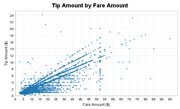
Relationship between tip amount and Fare Amount
        val plotDF = spark.sql("""
          SELECT fare_amount, passenger_count, tip_amount
          FROM tempView
          WHERE passenger_count > 0 AND passenger_count < 7 AND
                fare_amount > 0 AND fare_amount < 200 AND
                payment_type IN ('CSH', 'CRD') AND
                tip_amount > 0 AND tip_amount < 25
          LIMIT 10000
        """)
        val rows = plotDF.collect()
        val fareAmounts = rows.map(_.getAs[Double]("fare_amount"))
        val tipAmounts = rows.map(_.getAs[Double]("tip_amount"))
        val passengerCounts = rows.map(_.getAs[Double]("passenger_count"))
        val fig = Figure()
        val plt = fig.subplot(0)
        plt += plot(fareAmounts, tipAmounts, '.')

        plt.title = "Tip Amount by Fare Amount"
        plt.xlabel = "Fare Amount ($)"
        plt.ylabel = "Tip Amount ($)"
Output:
Feature engineering, transformation and data preparation for modeling
Next, we create a new feature tipped, if the tip_amount is non-zero, then this returns 1, else 0 in our case. We build a classifier with this target value later on.
        val sqlStatement = "Select *, " +
                  "CASE WHEN tip_amount > 0 THEN CAST(1.0 as Double) ELSE CAST(0.0 as Double) END AS tipped " +
                  "FROM tempView"
        val data_newFeature = spark.sql(sqlStatement)
        data_newFeature.show()
Output:
        +---------+---------------+-------------+---------+------------+-----------+----------+------+
        |vendor_id|passenger_count|trip_distance|rate_code|payment_type|fare_amount|tip_amount|tipped|
        +---------+---------------+-------------+---------+------------+-----------+----------+------+
        |      CMT|            1.0|          2.7|      1.0|         CSH|       14.0|       0.0|   0.0|
        |      CMT|            3.0|         20.4|      1.0|         CSH|       58.5|       0.0|   0.0|
        |      CMT|            1.0|          2.1|      1.0|         CSH|        9.5|       0.0|   0.0|
        |      CMT|            1.0|          1.3|      1.0|         CSH|        6.0|       0.0|   0.0|
        |      CMT|            2.0|          1.7|      1.0|         CSH|       10.5|       0.0|   0.0|
        |      CMT|            2.0|          1.7|      1.0|         CSH|       10.0|       0.0|   0.0|
        |      CMT|            1.0|          1.0|      1.0|         CSH|        6.0|       0.0|   0.0|
        |      CMT|            1.0|          9.2|      1.0|         CSH|       28.5|       0.0|   0.0|
        |      CMT|            1.0|          2.6|      1.0|         CSH|       11.5|       0.0|   0.0|
        |      CMT|            1.0|          1.4|      1.0|         CSH|        6.0|       0.0|   0.0|
        |      CMT|            4.0|          3.2|      1.0|         CSH|       13.0|       0.0|   0.0|
        |      CMT|            1.0|          7.8|      1.0|         CSH|       25.0|       0.0|   0.0|
        |      CMT|            1.0|          1.1|      1.0|         CSH|        5.5|       0.0|   0.0|
        |      CMT|            1.0|          3.3|      1.0|         CSH|       15.5|       0.0|   0.0|
        |      CMT|            1.0|          5.3|      1.0|         CSH|       19.5|       0.0|   0.0|
        |      CMT|            1.0|          6.2|      1.0|         CSH|       19.5|       0.0|   0.0|
        |      CMT|            1.0|         15.6|      2.0|         CSH|       52.0|       0.0|   0.0|
        |      CMT|            2.0|          0.9|      1.0|         CSH|        6.0|       0.0|   0.0|
        |      CMT|            1.0|          1.4|      1.0|         CSH|        9.0|       0.0|   0.0|
        |      CMT|            2.0|          1.2|      1.0|         CSH|        7.0|       0.0|   0.0|
        +---------+---------------+-------------+---------+------------+-----------+----------+------+
        only showing top 20 rows
Now, we figure out the average, minimum, maximum, etc. of columns, as this give us general idea about the range of values and other statistics. Apache Spark SQL provides us with a handy describe method that will help us to calculate these values.
data_newFeature.describe("passenger_count","trip_distance","rate_code","fare_amount","tip_amount").show()
Output:
        +-------+------------------+------------------+-------------------+------------------+------------------+
        |summary|   passenger_count|     trip_distance|          rate_code|       fare_amount|        tip_amount|
        +-------+------------------+------------------+-------------------+------------------+------------------+
        |  count|          12612051|          12612051|           12612051|          12612051|          12612051|
        |   mean| 1.711963105762893| 3.081084886986297| 1.0316361708337525|12.782634287634899|1.4699661752082924|
        | stddev|1.3616351834672402|3.6140504506213844|0.28838467968053266|10.461028944648847| 2.272277866399201|
        |    min|               1.0|              0.01|                0.0|               2.5|               0.0|
        |    max|               9.0|             100.0|              221.0|             500.0|             200.0|
        +-------+------------------+------------------+-------------------+------------------+------------------+
For modeling function from ML and MLlib, requires to prepare target and features by using a variety of techniques, such as indexing, one-hot encoding, and vectorization etc. Here are the procedures to follow in this section.
The dataset contains categorical fields: vendor_id, rate_code, and payment_type. Therefore, we need to convert these into indexed fields, because our models are mathematical and understand only numerical values.To do this, for indexing, we use StringIndexer(), and for one-hot encoding, use OneHotEncoder() functions. Here is the code to index and encode categorical features.
        val vendor_idIndexer = new StringIndexer()
          .setInputCol("vendor_id")
          .setOutputCol("vendor_idIndex")
        val Indexedvendor_id = vendor_idIndexer.fit(data_newFeature).transform(data_newFeature)
        //Indexedvendor_id.show()

        val vendor_idEncoder = new OneHotEncoder()
          .setInputCol("vendor_idIndex")
          .setOutputCol("vendor_idVec")
        val vendor_idEncoded = vendor_idEncoder.fit(Indexedvendor_id).transform(Indexedvendor_id)
        //vendor_idEncoded.show()

        val rate_codeIndexer = new StringIndexer()
          .setInputCol("rate_code")
          .setOutputCol("rate_codeIndex")
        val Indexedrate_code = rate_codeIndexer.fit(vendor_idEncoded).transform(vendor_idEncoded)

        val rate_codeEncoder = new OneHotEncoder()
          .setInputCol("rate_codeIndex")
          .setOutputCol("rate_codeVec")
        val rate_codeEncoded = rate_codeEncoder.fit(Indexedrate_code).transform(Indexedrate_code)
        //rate_codeEncoded.show()

        val payment_typeIndexer = new StringIndexer()
          .setInputCol("payment_type")
          .setOutputCol("payment_typeIndex")
        val Indexedpayment_type = payment_typeIndexer.fit(rate_codeEncoded).transform(rate_codeEncoded)

        val payment_typeEncoder = new OneHotEncoder()
          .setInputCol("payment_typeIndex")
          .setOutputCol("payment_typeVec")
        val FinalEncoded = payment_typeEncoder.fit(Indexedpayment_type).transform(Indexedpayment_type)
        FinalEncoded.show()
Output:
        +---------+---------------+-------------+---------+------------+-----------+----------+------+--------------+------------+--------------+--------------+-----------------+---------------+
        |vendor_id|passenger_count|trip_distance|rate_code|payment_type|fare_amount|tip_amount|tipped|vendor_idIndex|vendor_idVec|rate_codeIndex|  rate_codeVec|payment_typeIndex|payment_typeVec|
        +---------+---------------+-------------+---------+------------+-----------+----------+------+--------------+------------+--------------+--------------+-----------------+---------------+
        |      CMT|            1.0|          2.7|      1.0|         CSH|       14.0|       0.0|   0.0|           1.0|   (1,[],[])|           0.0|(11,[0],[1.0])|              1.0|  (4,[1],[1.0])|
        |      CMT|            3.0|         20.4|      1.0|         CSH|       58.5|       0.0|   0.0|           1.0|   (1,[],[])|           0.0|(11,[0],[1.0])|              1.0|  (4,[1],[1.0])|
        |      CMT|            1.0|          2.1|      1.0|         CSH|        9.5|       0.0|   0.0|           1.0|   (1,[],[])|           0.0|(11,[0],[1.0])|              1.0|  (4,[1],[1.0])|
        |      CMT|            1.0|          1.3|      1.0|         CSH|        6.0|       0.0|   0.0|           1.0|   (1,[],[])|           0.0|(11,[0],[1.0])|              1.0|  (4,[1],[1.0])|
        |      CMT|            2.0|          1.7|      1.0|         CSH|       10.5|       0.0|   0.0|           1.0|   (1,[],[])|           0.0|(11,[0],[1.0])|              1.0|  (4,[1],[1.0])|
        |      CMT|            2.0|          1.7|      1.0|         CSH|       10.0|       0.0|   0.0|           1.0|   (1,[],[])|           0.0|(11,[0],[1.0])|              1.0|  (4,[1],[1.0])|
        |      CMT|            1.0|          1.0|      1.0|         CSH|        6.0|       0.0|   0.0|           1.0|   (1,[],[])|           0.0|(11,[0],[1.0])|              1.0|  (4,[1],[1.0])|
        |      CMT|            1.0|          9.2|      1.0|         CSH|       28.5|       0.0|   0.0|           1.0|   (1,[],[])|           0.0|(11,[0],[1.0])|              1.0|  (4,[1],[1.0])|
        |      CMT|            1.0|          2.6|      1.0|         CSH|       11.5|       0.0|   0.0|           1.0|   (1,[],[])|           0.0|(11,[0],[1.0])|              1.0|  (4,[1],[1.0])|
        |      CMT|            1.0|          1.4|      1.0|         CSH|        6.0|       0.0|   0.0|           1.0|   (1,[],[])|           0.0|(11,[0],[1.0])|              1.0|  (4,[1],[1.0])|
        |      CMT|            4.0|          3.2|      1.0|         CSH|       13.0|       0.0|   0.0|           1.0|   (1,[],[])|           0.0|(11,[0],[1.0])|              1.0|  (4,[1],[1.0])|
        |      CMT|            1.0|          7.8|      1.0|         CSH|       25.0|       0.0|   0.0|           1.0|   (1,[],[])|           0.0|(11,[0],[1.0])|              1.0|  (4,[1],[1.0])|
        |      CMT|            1.0|          1.1|      1.0|         CSH|        5.5|       0.0|   0.0|           1.0|   (1,[],[])|           0.0|(11,[0],[1.0])|              1.0|  (4,[1],[1.0])|
        |      CMT|            1.0|          3.3|      1.0|         CSH|       15.5|       0.0|   0.0|           1.0|   (1,[],[])|           0.0|(11,[0],[1.0])|              1.0|  (4,[1],[1.0])|
        |      CMT|            1.0|          5.3|      1.0|         CSH|       19.5|       0.0|   0.0|           1.0|   (1,[],[])|           0.0|(11,[0],[1.0])|              1.0|  (4,[1],[1.0])|
        |      CMT|            1.0|          6.2|      1.0|         CSH|       19.5|       0.0|   0.0|           1.0|   (1,[],[])|           0.0|(11,[0],[1.0])|              1.0|  (4,[1],[1.0])|
        |      CMT|            1.0|         15.6|      2.0|         CSH|       52.0|       0.0|   0.0|           1.0|   (1,[],[])|           1.0|(11,[1],[1.0])|              1.0|  (4,[1],[1.0])|
        |      CMT|            2.0|          0.9|      1.0|         CSH|        6.0|       0.0|   0.0|           1.0|   (1,[],[])|           0.0|(11,[0],[1.0])|              1.0|  (4,[1],[1.0])|
        |      CMT|            1.0|          1.4|      1.0|         CSH|        9.0|       0.0|   0.0|           1.0|   (1,[],[])|           0.0|(11,[0],[1.0])|              1.0|  (4,[1],[1.0])|
        |      CMT|            2.0|          1.2|      1.0|         CSH|        7.0|       0.0|   0.0|           1.0|   (1,[],[])|           0.0|(11,[0],[1.0])|              1.0|  (4,[1],[1.0])|
        +---------+---------------+-------------+---------+------------+-----------+----------+------+--------------+------------+--------------+--------------+-----------------+---------------+
        only showing top 20 rows
This code creates a 25% random sampling of the data in this example. Next, split the sample into a training part (75%, in this example) and a testing part (25%, in this example) to use in classification and regression modeling.
        val sampleingFraction = 0.25
        val trainingFraction = 0.75
        val testingFraction = (1 - trainingFraction)
        val seed = 1234

        val FinalSampled = FinalEncoded.sample(withReplacement = false, fraction = sampleingFraction, seed = seed)

        val splits = FinalSampled.randomSplit(Array(trainingFraction, testingFraction), seed=seed)
        val trainData = splits(0)
        val testData = splits(1)
Now, we use VectorAssembler which is a transformer that combines a given list of columns into a single vector column. It is useful for combining raw features and features generated by different feature transformers into a single feature vector, in order to train ML models, VectorAssembler accepts the input column, in each row, the values of the input columns will be concatenated into a vector in the specified order.
        val va = new VectorAssembler().setInputCols(
          Array("vendor_idVec","rate_codeVec","payment_typeVec","passenger_count","trip_distance","fare_amount"))
          .setOutputCol("features")

        val oneHotTrain = va.transform(trainData)
        val oneHotTest = va.transform(testData)
        oneHotTrain.show()
        +---------+---------------+-------------+---------+------------+-----------+----------+------+--------------+------------+--------------+--------------+-----------------+---------------+--------------------+
        |vendor_id|passenger_count|trip_distance|rate_code|payment_type|fare_amount|tip_amount|tipped|vendor_idIndex|vendor_idVec|rate_codeIndex|  rate_codeVec|payment_typeIndex|payment_typeVec|            features|
        +---------+---------------+-------------+---------+------------+-----------+----------+------+--------------+------------+--------------+--------------+-----------------+---------------+--------------------+
        |      CMT|            1.0|          0.1|      1.0|         CRD|        2.5|       0.1|   1.0|           1.0|   (1,[],[])|           0.0|(11,[0],[1.0])|              0.0|  (4,[0],[1.0])|(19,[1,12,16,17,1...|
        |      CMT|            1.0|          0.1|      1.0|         CRD|        2.5|       1.0|   1.0|           1.0|   (1,[],[])|           0.0|(11,[0],[1.0])|              0.0|  (4,[0],[1.0])|(19,[1,12,16,17,1...|
        |      CMT|            1.0|          0.1|      1.0|         CRD|        3.0|       0.0|   0.0|           1.0|   (1,[],[])|           0.0|(11,[0],[1.0])|              0.0|  (4,[0],[1.0])|(19,[1,12,16,17,1...|
        |      CMT|            1.0|          0.1|      1.0|         CRD|        3.0|       0.5|   1.0|           1.0|   (1,[],[])|           0.0|(11,[0],[1.0])|              0.0|  (4,[0],[1.0])|(19,[1,12,16,17,1...|
        |      CMT|            1.0|          0.1|      1.0|         CRD|        3.0|       0.7|   1.0|           1.0|   (1,[],[])|           0.0|(11,[0],[1.0])|              0.0|  (4,[0],[1.0])|(19,[1,12,16,17,1...|
        |      CMT|            1.0|          0.1|      1.0|         CRD|        3.0|       0.7|   1.0|           1.0|   (1,[],[])|           0.0|(11,[0],[1.0])|              0.0|  (4,[0],[1.0])|(19,[1,12,16,17,1...|
        |      CMT|            1.0|          0.1|      1.0|         CRD|        3.0|       0.8|   1.0|           1.0|   (1,[],[])|           0.0|(11,[0],[1.0])|              0.0|  (4,[0],[1.0])|(19,[1,12,16,17,1...|
        |      CMT|            1.0|          0.1|      1.0|         CRD|        3.0|       0.8|   1.0|           1.0|   (1,[],[])|           0.0|(11,[0],[1.0])|              0.0|  (4,[0],[1.0])|(19,[1,12,16,17,1...|
        |      CMT|            1.0|          0.1|      1.0|         CRD|        3.0|       0.8|   1.0|           1.0|   (1,[],[])|           0.0|(11,[0],[1.0])|              0.0|  (4,[0],[1.0])|(19,[1,12,16,17,1...|
        |      CMT|            1.0|          0.1|      1.0|         CRD|        3.0|      1.05|   1.0|           1.0|   (1,[],[])|           0.0|(11,[0],[1.0])|              0.0|  (4,[0],[1.0])|(19,[1,12,16,17,1...|
        |      CMT|            1.0|          0.1|      1.0|         CRD|        3.0|       3.0|   1.0|           1.0|   (1,[],[])|           0.0|(11,[0],[1.0])|              0.0|  (4,[0],[1.0])|(19,[1,12,16,17,1...|
        |      CMT|            1.0|          0.1|      1.0|         CRD|        3.0|       3.0|   1.0|           1.0|   (1,[],[])|           0.0|(11,[0],[1.0])|              0.0|  (4,[0],[1.0])|(19,[1,12,16,17,1...|
        |      CMT|            1.0|          0.1|      1.0|         CRD|        3.5|       1.0|   1.0|           1.0|   (1,[],[])|           0.0|(11,[0],[1.0])|              0.0|  (4,[0],[1.0])|(19,[1,12,16,17,1...|
        |      CMT|            1.0|          0.1|      1.0|         CRD|        4.0|       1.1|   1.0|           1.0|   (1,[],[])|           0.0|(11,[0],[1.0])|              0.0|  (4,[0],[1.0])|(19,[1,12,16,17,1...|
        |      CMT|            1.0|          0.1|      1.0|         CSH|        2.5|       0.0|   0.0|           1.0|   (1,[],[])|           0.0|(11,[0],[1.0])|              1.0|  (4,[1],[1.0])|(19,[1,13,16,17,1...|
        |      CMT|            1.0|          0.1|      1.0|         CSH|        2.5|       0.0|   0.0|           1.0|   (1,[],[])|           0.0|(11,[0],[1.0])|              1.0|  (4,[1],[1.0])|(19,[1,13,16,17,1...|
        |      CMT|            1.0|          0.1|      1.0|         CSH|        2.5|       0.0|   0.0|           1.0|   (1,[],[])|           0.0|(11,[0],[1.0])|              1.0|  (4,[1],[1.0])|(19,[1,13,16,17,1...|
        |      CMT|            1.0|          0.1|      1.0|         CSH|        2.5|       0.0|   0.0|           1.0|   (1,[],[])|           0.0|(11,[0],[1.0])|              1.0|  (4,[1],[1.0])|(19,[1,13,16,17,1...|
        |      CMT|            1.0|          0.1|      1.0|         CSH|        2.5|       0.0|   0.0|           1.0|   (1,[],[])|           0.0|(11,[0],[1.0])|              1.0|  (4,[1],[1.0])|(19,[1,13,16,17,1...|
        |      CMT|            1.0|          0.1|      1.0|         CSH|        2.5|       0.0|   0.0|           1.0|   (1,[],[])|           0.0|(11,[0],[1.0])|              1.0|  (4,[1],[1.0])|(19,[1,13,16,17,1...|
        +---------+---------------+-------------+---------+------------+-----------+----------+------+--------------+------------+--------------+--------------+-----------------+---------------+--------------------+
        only showing top 20 rows
Classification
Logistic Regression Model:
Logistic regression is a popular method to predict a categorical response. It is a special case of
Generalized Linear models that predicts the probability of the outcomes. In spark.ml logistic
regression can be used to predict a binary outcome by using binomial logistic regression. In this
section, we create binary classificaton model to predict whether or not a tip should be paid.
        val lr_logistic = new LogisticRegression()
            .setLabelCol("tipped")
            .setFeaturesCol("features")
            .setMaxIter(10)
            .setRegParam(0.3)
            .setElasticNetParam(0.8)

        val lrModel_logistic = lr_logistic.fit(oneHotTrain)
        val predictions_logistic = lrModel_logistic.transform(oneHotTest)
        predictions_logistic.show()
Output:
        +---------+---------------+-------------+---------+------------+-----------+----------+------+--------------+------------+--------------+--------------+-----------------+---------------+--------------------+--------------------+--------------------+----------+
        |vendor_id|passenger_count|trip_distance|rate_code|payment_type|fare_amount|tip_amount|tipped|vendor_idIndex|vendor_idVec|rate_codeIndex|  rate_codeVec|payment_typeIndex|payment_typeVec|            features|       rawPrediction|         probability|prediction|
        +---------+---------------+-------------+---------+------------+-----------+----------+------+--------------+------------+--------------+--------------+-----------------+---------------+--------------------+--------------------+--------------------+----------+
        |      CMT|            1.0|          0.1|      1.0|         CRD|        2.5|       0.6|   1.0|           1.0|   (1,[],[])|           0.0|(11,[0],[1.0])|              0.0|  (4,[0],[1.0])|(19,[1,12,16,17,1...|[-1.0014127011561...|[0.26866375814468...|       1.0|
        |      CMT|            1.0|          0.1|      1.0|         CRD|        3.0|       0.0|   0.0|           1.0|   (1,[],[])|           0.0|(11,[0],[1.0])|              0.0|  (4,[0],[1.0])|(19,[1,12,16,17,1...|[-1.0014127011561...|[0.26866375814468...|       1.0|
        |      CMT|            1.0|          0.1|      1.0|         CSH|        2.5|       0.0|   0.0|           1.0|   (1,[],[])|           0.0|(11,[0],[1.0])|              1.0|  (4,[1],[1.0])|(19,[1,13,16,17,1...|[0.79887452857404...|[0.68973368041605...|       0.0|
        |      CMT|            1.0|          0.1|      1.0|         CSH|        2.5|       0.0|   0.0|           1.0|   (1,[],[])|           0.0|(11,[0],[1.0])|              1.0|  (4,[1],[1.0])|(19,[1,13,16,17,1...|[0.79887452857404...|[0.68973368041605...|       0.0|
        |      CMT|            1.0|          0.1|      1.0|         CSH|        2.5|       0.0|   0.0|           1.0|   (1,[],[])|           0.0|(11,[0],[1.0])|              1.0|  (4,[1],[1.0])|(19,[1,13,16,17,1...|[0.79887452857404...|[0.68973368041605...|       0.0|
        |      CMT|            1.0|          0.1|      1.0|         CSH|        2.5|       0.0|   0.0|           1.0|   (1,[],[])|           0.0|(11,[0],[1.0])|              1.0|  (4,[1],[1.0])|(19,[1,13,16,17,1...|[0.79887452857404...|[0.68973368041605...|       0.0|
        |      CMT|            1.0|          0.1|      1.0|         CSH|        2.5|       0.0|   0.0|           1.0|   (1,[],[])|           0.0|(11,[0],[1.0])|              1.0|  (4,[1],[1.0])|(19,[1,13,16,17,1...|[0.79887452857404...|[0.68973368041605...|       0.0|
        |      CMT|            1.0|          0.1|      1.0|         CSH|        2.5|       0.0|   0.0|           1.0|   (1,[],[])|           0.0|(11,[0],[1.0])|              1.0|  (4,[1],[1.0])|(19,[1,13,16,17,1...|[0.79887452857404...|[0.68973368041605...|       0.0|
        |      CMT|            1.0|          0.1|      1.0|         CSH|        2.5|       0.0|   0.0|           1.0|   (1,[],[])|           0.0|(11,[0],[1.0])|              1.0|  (4,[1],[1.0])|(19,[1,13,16,17,1...|[0.79887452857404...|[0.68973368041605...|       0.0|
        |      CMT|            1.0|          0.1|      1.0|         CSH|        2.5|       0.0|   0.0|           1.0|   (1,[],[])|           0.0|(11,[0],[1.0])|              1.0|  (4,[1],[1.0])|(19,[1,13,16,17,1...|[0.79887452857404...|[0.68973368041605...|       0.0|
        |      CMT|            1.0|          0.1|      1.0|         CSH|        2.5|       0.0|   0.0|           1.0|   (1,[],[])|           0.0|(11,[0],[1.0])|              1.0|  (4,[1],[1.0])|(19,[1,13,16,17,1...|[0.79887452857404...|[0.68973368041605...|       0.0|
        |      CMT|            1.0|          0.1|      1.0|         CSH|        2.5|       0.0|   0.0|           1.0|   (1,[],[])|           0.0|(11,[0],[1.0])|              1.0|  (4,[1],[1.0])|(19,[1,13,16,17,1...|[0.79887452857404...|[0.68973368041605...|       0.0|
        |      CMT|            1.0|          0.1|      1.0|         CSH|        2.5|       0.0|   0.0|           1.0|   (1,[],[])|           0.0|(11,[0],[1.0])|              1.0|  (4,[1],[1.0])|(19,[1,13,16,17,1...|[0.79887452857404...|[0.68973368041605...|       0.0|
        |      CMT|            1.0|          0.1|      1.0|         CSH|        2.5|       0.0|   0.0|           1.0|   (1,[],[])|           0.0|(11,[0],[1.0])|              1.0|  (4,[1],[1.0])|(19,[1,13,16,17,1...|[0.79887452857404...|[0.68973368041605...|       0.0|
        |      CMT|            1.0|          0.1|      1.0|         CSH|        3.0|       0.0|   0.0|           1.0|   (1,[],[])|           0.0|(11,[0],[1.0])|              1.0|  (4,[1],[1.0])|(19,[1,13,16,17,1...|[0.79887452857404...|[0.68973368041605...|       0.0|
        |      CMT|            1.0|          0.1|      1.0|         CSH|        3.0|       0.0|   0.0|           1.0|   (1,[],[])|           0.0|(11,[0],[1.0])|              1.0|  (4,[1],[1.0])|(19,[1,13,16,17,1...|[0.79887452857404...|[0.68973368041605...|       0.0|
        |      CMT|            1.0|          0.1|      1.0|         CSH|        3.0|       0.0|   0.0|           1.0|   (1,[],[])|           0.0|(11,[0],[1.0])|              1.0|  (4,[1],[1.0])|(19,[1,13,16,17,1...|[0.79887452857404...|[0.68973368041605...|       0.0|
        |      CMT|            1.0|          0.1|      1.0|         CSH|        3.0|       0.0|   0.0|           1.0|   (1,[],[])|           0.0|(11,[0],[1.0])|              1.0|  (4,[1],[1.0])|(19,[1,13,16,17,1...|[0.79887452857404...|[0.68973368041605...|       0.0|
        |      CMT|            1.0|          0.1|      1.0|         CSH|        3.0|       0.0|   0.0|           1.0|   (1,[],[])|           0.0|(11,[0],[1.0])|              1.0|  (4,[1],[1.0])|(19,[1,13,16,17,1...|[0.79887452857404...|[0.68973368041605...|       0.0|
        |      CMT|            1.0|          0.1|      1.0|         CSH|        3.0|       0.0|   0.0|           1.0|   (1,[],[])|           0.0|(11,[0],[1.0])|              1.0|  (4,[1],[1.0])|(19,[1,13,16,17,1...|[0.79887452857404...|[0.68973368041605...|       0.0|
        +---------+---------------+-------------+---------+------------+-----------+----------+------+--------------+------------+--------------+--------------+-----------------+---------------+--------------------+--------------------+--------------------+----------+
        only showing top 20 rows
Now, we print the coefficients and intercept for logistic regression, use BinaryClassificationEvaluator() to compute error. We also create evaluators for multiclass and binary classification.
        val evaluator_logistic = new BinaryClassificationEvaluator()
          .setLabelCol("tipped")
          .setRawPredictionCol("probability")
          .setMetricName("areaUnderROC")
        val ROC = evaluator_logistic.evaluate(predictions_logistic)

        println(s"Coefficients: ${lrModel_logistic.coefficients} Intercept: ${lrModel_logistic.intercept}")

       val evaluatorMC = new MulticlassClassificationEvaluator()
          .setLabelCol("tipped")
          .setPredictionCol("prediction")

        val evaluatorBC = new BinaryClassificationEvaluator()
          .setLabelCol("tipped")
          .setRawPredictionCol("probability")

        evaluatorMC.setMetricName("accuracy")
        println("Accuracy = " + evaluatorMC.evaluate(predictions_logistic))

        evaluatorMC.setMetricName("f1")
        println("F1 Score = " + evaluatorMC.evaluate(predictions_logistic))

        evaluatorMC.setMetricName("weightedPrecision")
        println("Weighted Precision = " + evaluatorMC.evaluate(predictions_logistic))

        evaluatorMC.setMetricName("weightedRecall")
        println("Weighted Recall = " + evaluatorMC.evaluate(predictions_logistic))

        evaluatorBC.setMetricName("areaUnderROC")
        println("Area Under ROC = " + evaluatorBC.evaluate(predictions_logistic))

        evaluatorBC.setMetricName("areaUnderPR")
        println("Area Under PR = " + evaluatorBC.evaluate(predictions_logistic))

        evaluatorMC.setMetricName("truePositiveRateByLabel")
        println("True Positive Rate = " + evaluatorMC.evaluate(predictions_logistic))

        evaluatorMC.setMetricName("falsePositiveRateByLabel")
        println("False Positive Rate = " + evaluatorMC.evaluate(predictions_logistic))
Output:
        Coefficients: (19,[12,13],[0.8683140968749369,-0.9319731328552421]) Intercept: 0.13309860428112388
        Accuracy = 0.9757668606619853
        F1 Score = 0.9756927081729325
        Weighted Precision = 0.9767875098709558
        Weighted Recall = 0.9757668606619853
        Area Under ROC = 0.9761832349547527
        Area Under PR = 0.962533188519613
        True Positive Rate = 0.9461586599989852
        False Positive Rate = 1.8443336307321312E-5
A confusion matrix for binary classification is a 2x2 table that summarizes a classifier's
performance by comparing its predicted outcomes against the actual outcomes. It contains
four key metrics:
Ture Positive(TP), False Positives (FP), True Negatives (TN), and
False Negatives (FN),
which represent the counts of correct and incorrect predictions for each class.
True Positive (TP)
: The number of instances that were correctly predicted as the positive class.
False Positive (FP)
: The number of instances that were incorrectly predicted as the positive class when they
were actually negative
True Negative (TN)
: The number of instances that were correctly predicted as the negative class.
False Negative (FN)
: The number of instances that were incorrectly predicted as the negative class when they were actually positive.
        val confusionMatrix = predictions_logistic
        .groupBy("tipped", "prediction")
        .count()
        .orderBy("tipped", "prediction")

        println("Confusion Matrix:")
        confusionMatrix.show()
        Confusion Matrix:
        +------+----------+------+
        |tipped|prediction| count|
        +------+----------+------+
        |   0.0|       0.0|335646|
        |   0.0|       1.0| 19100|
        |   1.0|       0.0|     8|
        |   1.0|       1.0|433753|
        +------+----------+------+
We calculate TP, TN, FP, FN manually
        val tp = predictions_logistic.filter(col("tipped") === 1.0 && col("prediction") === 1.0).count()
        val tn = predictions_logistic.filter(col("tipped") === 0.0 && col("prediction") === 0.0).count()
        val fp = predictions_logistic.filter(col("tipped") === 0.0 && col("prediction") === 1.0).count()
        val fn = predictions_logistic.filter(col("tipped") === 1.0 && col("prediction") === 0.0).count()

        println(s"True Positives: $tp")
        println(s"True Negatives: $tn")
        println(s"False Positives: $fp")
        println(s"False Negatives: $fn")

        // Calculate additional metrics
        val total = predictions_logistic.count().toDouble
        val accuracyManual = (tp + tn) / total
        val precision = tp.toDouble / (tp + fp)
        val recall = tp.toDouble / (tp + fn)
        val f1ScoreManual = 2 * (precision * recall) / (precision + recall)

        println(s"Manual Accuracy: $accuracyManual")
        println(s"Precision: $precision")
        println(s"Recall: $recall")
        println(s"Manual F1 Score: $f1ScoreManual")
        True Positives: 433753
        True Negatives: 335646
        False Positives: 19100
        False Negatives: 8
        Manual Accuracy: 0.9757668606619853
        Precision: 0.957822958001824
        Recall: 0.9999815566636927
        Manual F1 Score: 0.978448343924188
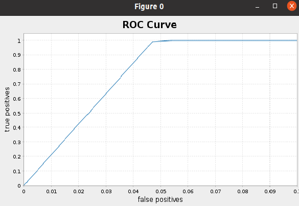
Now, We are intested to plot ROC Curve and run the code following
        val BM = new BinaryClassificationMetrics(predictions_logistic.select(col("probability"), col("tipped"))
        .rdd.map(r=>(r.getAs[DenseVector](0)(1),(r.getDouble(1)))))

        val roc = BM.roc().collect()
        //roc.foreach{println}
        val falsePositives = roc.map{ _._1 }
        val truePositives = roc.map{ _._2 }
        val f = Figure()
        val p = f.subplot(0)
        p += plot(falsePositives, truePositives)
        p.xlabel = "false positives"
        p.ylabel = "true positives"
        p.xlim(0.0, 0.1)
        p.xaxis.setTickUnit(new NumberTickUnit(0.01))
        p.yaxis.setTickUnit(new NumberTickUnit(0.1))
        p.title="ROC Curve"
        f.refresh()
Regression
Linear Regression Model:
In this section, we will create Linear Regression Model to predict the tip amount. Now,
we create linear regression model by using Spark ML functions and fit the model
with training dataset and then print the coefficients and intercept for linear regression.
        val lr_linear = new LinearRegression()
          .setLabelCol("tip_amount")
          .setFeaturesCol("features")
          .setMaxIter(10)
          .setRegParam(0.3)
          .setElasticNetParam(0.8)

        val lrModel_linear = lr_linear.fit(oneHotTrain)

        println(s"Coefficients: ${lrModel_linear.coefficients} Intercept: ${lrModel_linear.intercept}")
Output:
Coefficients: [0.0,0.0,0.0,0.0,0.0,0.0,0.0,0.0,0.0,0.0,0.0,0.0,0.9744213718064276,-0.9745531398802871,0.0,0.0,0.0,0.054476496827110324,0.06383384569576009] Intercept: 0.3475394768937951
Next, summarize the model over the training set and print out some metrics
        val trainingSummary = lrModel_linear.summary
        println(s"numIterations: ${trainingSummary.totalIterations}")
        println(s"objectiveHistory: [${trainingSummary.objectiveHistory.mkString(",")}]")
Output:
        numIterations: 10
        objectiveHistory: [0.4999999999999999,0.4669433877959451,0.32939485958509823,0.32699194111858804,0.3260201539767395,0.3258501608715561,0.32578643813382124,0.3257455699728877,0.32562545716988356,0.32543634215625095,0.325428544351327]
Summary residuals
trainingSummary.residuals.show()
Output:
        +--------------------+
        |           residuals|
        +--------------------+
        |  -1.386993112622334|
        |-0.48699311262233413|
        |  -1.518910035470214|
        |  -1.018910035470214|
        | -0.8189100354702141|
        | -0.8189100354702141|
        |  -0.718910035470214|
        |  -0.718910035470214|
        |  -0.718910035470214|
        |-0.46891003547021404|
        |   1.481089964529786|
        |   1.481089964529786|
        | -0.5508269583180943|
        | -0.4827438811659741|
        |  0.4619813990643807|
        |  0.4619813990643807|
        |  0.4619813990643807|
        |  0.4619813990643807|
        |  0.4619813990643807|
        |  0.4619813990643807|
        +--------------------+
        only showing top 20 rows
RMSC and r2.
        println(s"RMSE: ${trainingSummary.rootMeanSquaredError}")
        println(s"r2: ${trainingSummary.r2}")
Output:
        RMSE: 1.5685565413144988
        r2: 0.5239750266508932
Finally, We score and evaluate the model on test data.
        val predictions_linear = lrModel_linear.transform(oneHotTest)
        //predictions_linear.show()

        val evaluator_linear = new RegressionEvaluator()
          .setLabelCol("tip_amount")
          .setPredictionCol("prediction")
          .setMetricName("r2")
        val r2_linear = evaluator_linear.evaluate(predictions_linear)

        println("R-sqr on test data = " + r2_linear)
Output:
R-sqr on test data = 0.525914213006671
However, it is still possible to increase the accuracy by performing Cross-Validation and hyperparameter tunning.
• References
• Big Data Analytics with Java by Rajat Mehta.
• The home for Microsoft documentation and learning for developers and technology professionals. docs.microsoft.com.
• And Others.
Image:freepik